6.线性回归——单变量梯度下降算法的实现

权重和偏执的更新公式：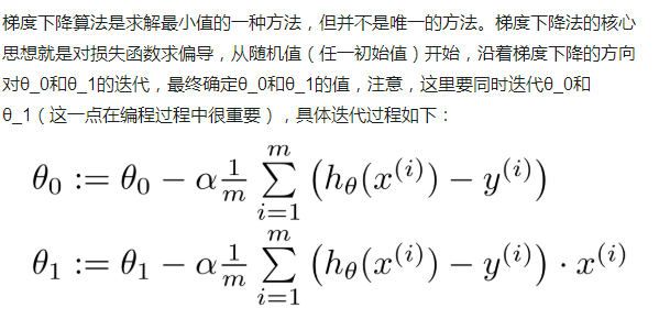

import numpy as np 
import matplotlib.pyplot as plt 

def readData(path):
	data = np.loadtxt(path,dtype = float,delimiter = ",")
	return data

def costFunction(theta_0,theta_1,x,y,m):
	predictValue = theta_1 * x + theta_0
	return sum((predictValue - y) ** 2)/(2 * m)

def gradientDescent(data,theta_0,theta_1,iterations,alpha):
	eachIterationValue = np.zeros((iterations,1))
	#iterations 行，1列
	x = data[:,0]  #第0列
	y = data[:,1]  #第1列
	m = data.shape[0]  #data.shape[0]表示行数
	for i in range(0,iterations):
		hypothesis = theta_1 * x + theta_0
		temp_0 = theta_0 - alpha * ((1/m) * sum(hypothesis - y))
		#更新偏执 theta_0
		temp_1 = theta_1 - alpha * (1/m) * sum ((hypothesis - y) * x)
		#更新权重 theta_1
		theta_0 = temp_0
		theta_1 = temp_1
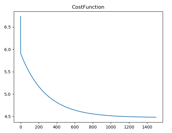
		costFunction_temp = costFunction(theta_0,theta_1,x,y,m)
		eachIterationValue[i,0] = costFunction_temp
		#依次列出损失函数的值

	return theta_0,theta_1,eachIterationValue

if __name__ == '__main__':
	data = readData('ex1data1.txt')
	iterations = 1500
	plt.scatter(data[:,0],data[:,1],color = 'g',s = 20)
	theta_0,theta_1,eachIterationValue = gradientDescent(data,0,0,iterations,0.01)
	hypothesis = theta_1 * data[:,0]  + theta_0
	plt.plot(data[:,0],hypothesis)
	plt.title('Fittingcurve')
	plt.show()
	plt.plot(np.arange(iterations),eachIterationValue)
	plt.title('CostFunction')
	plt.show()

运算结果：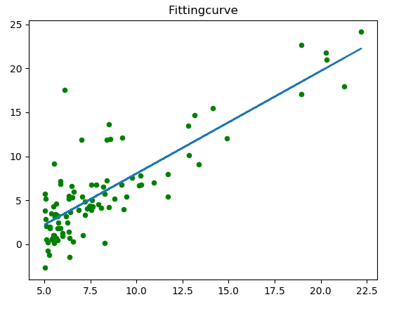

参考： https://www.imooc.com/article/252827
数据集链接：链接：https://pan.baidu.com/s/1u8ln5I-Ejfg6O7Xv06paAA
提取码：rr76