
用深度学习处理文本数据
6.1 Working with text data
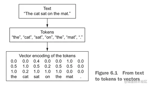
要用深度学习的神经网络处理文本数据,和图片类似,也要把数据向量化:文本 -> 数值张量。
要做这种事情可以把每个单词变成向量,也可以把字符变成向量,还可以把多个连续单词或字符(称为 N-grams)变成向量。
反正不管如何划分,我们把文本拆分出来的单元叫做 tokens(标记),拆分文本的过程叫做 tokenization(分词)。
注:token 这个词在很多中文翻译里都是“标记”。我觉得这个翻译都怪怪的,虽然 token 确实有「标记」这个意思,但我觉得 token 翻译成“标记”就没内味儿了。我理解的 token 是那种「可以代表另一个东西来在特定场景中使用的东西」,是一种有实体的东西,这种意义更接近于「代金券」、「代币」。
文本的向量化就是先作分词,然后把生成出来的 token 逐个与数值向量对应起来,最后拿对应的数值向量合成一个表达了原文本的张量。其中,比较有意思的是如何建立 token 和 数值向量 的联系,下面介绍两种搞这个的方法:one-hot encoding(one-hot编码) 和 token embedding(标记嵌入),其中 token embedding 一般都用于单词,叫作词嵌入「word embedding」。
n-grams 和词袋(bag-of-words)
n-gram 是能从一个句子中提取出的 ≤N 个连续单词的集合。例如:「The cat sat on the mat.」
这个句子分解成 2-gram 是:
{"The", "The cat", "cat", "cat sat", "sat",
"sat on", "on", "on the", "the", "the mat", "mat"}
这个集合被叫做 bag-of-2-grams (二元语法袋)。
分解成 3-gram 是:
{"The", "The cat", "cat", "cat sat", "The cat sat",
"sat", "sat on", "on", "cat sat on", "on the", "the",
"sat on the", "the mat", "mat", "on the mat"}
这个集合被叫做 bag-of-3-grams (三元语法袋)。
把这东西叫做「袋」是因为它只是 tokens 组成的集合,没有原来文本的顺序和意义。把文本分成这种袋的分词方法叫做「词袋(bag-of-words)」。
由于词袋是不保存顺序的(分出来是集合,不是序列),所以一般不在深度学习里面用。但在轻量级的浅层文本处理模型里面,n-gram 和词袋还是很重要的方法的。
one-hot 编码
one-hot 是比较基本、常用的。其做法是将每个 token 与一个唯一整数索引关联, 然后将整数索引 i 转换为长度为 N 的二进制向量(N 是词表大小),这个向量只有第 i 个元素为 1,其余元素都为 0。
下面给出两个玩具版本的 one-hot 编码示例:
# 单词级的 one-hot 编码
import numpy as np
samples = ['The cat sat on the mat.', 'The dog ate my homework.']
token_index = {}
for sample in samples:
for word in sample.split():
if word not in token_index:
token_index[word] = len(token_index) + 1
# 对样本进行分词。只考虑每个样本前 max_length 个单词
max_length = 10
results = np.zeros(shape=(len(samples),
max_length,
max(token_index.values()) + 1))
for i, sample in enumerate(samples):
for j, word in list(enumerate(sample.split()))[:max_length]:
index = token_index.get(word)
results[i, j, index] = 1.
print(results)
[[[0. 1. 0. 0. 0. 0. 0. 0. 0. 0. 0.]
[0. 0. 1. 0. 0. 0. 0. 0. 0. 0. 0.]
[0. 0. 0. 1. 0. 0. 0. 0. 0. 0. 0.]
[0. 0. 0. 0. 1. 0. 0. 0. 0. 0. 0.]
[0. 0. 0. 0. 0. 1. 0. 0. 0. 0. 0.]
[0. 0. 0. 0. 0. 0. 1. 0. 0. 0. 0.]
[0. 0. 0. 0. 0. 0. 0. 0. 0. 0. 0.]
[0. 0. 0. 0. 0. 0. 0. 0. 0. 0. 0.]
[0. 0. 0. 0. 0. 0. 0. 0. 0. 0. 0.]
[0. 0. 0. 0. 0. 0. 0. 0. 0. 0. 0.]]
[[0. 1. 0. 0. 0. 0. 0. 0. 0. 0. 0.]
[0. 0. 0. 0. 0. 0. 0. 1. 0. 0. 0.]
[0. 0. 0. 0. 0. 0. 0. 0. 1. 0. 0.]
[0. 0. 0. 0. 0. 0. 0. 0. 0. 1. 0.]
[0. 0. 0. 0. 0. 0. 0. 0. 0. 0. 1.]
[0. 0. 0. 0. 0. 0. 0. 0. 0. 0. 0.]
[0. 0. 0. 0. 0. 0. 0. 0. 0. 0. 0.]
[0. 0. 0. 0. 0. 0. 0. 0. 0. 0. 0.]
[0. 0. 0. 0. 0. 0. 0. 0. 0. 0. 0.]
[0. 0. 0. 0. 0. 0. 0. 0. 0. 0. 0.]]]
# 字符级的 one-hot 编码
import string
samples = ['The cat sat on the mat.', 'The dog ate my homework.']
characters = string.printable # 所有可打印的 ASCII 字符
token_index = dict(zip(range(1, len(characters) + 1), characters))
max_length = 50
results = np.zeros((len(samples), max_length, max(token_index.keys()) + 1))
for i, sample in enumerate(samples):
for j, character in enumerate(sample):
index = token_index.get(character)
results[i, j, index] = 1.
print(results)
[[[1. 1. 1. ... 1. 1. 1.]
[1. 1. 1. ... 1. 1. 1.]
[1. 1. 1. ... 1. 1. 1.]
...
[0. 0. 0. ... 0. 0. 0.]
[0. 0. 0. ... 0. 0. 0.]
[0. 0. 0. ... 0. 0. 0.]]
[[1. 1. 1. ... 1. 1. 1.]
[1. 1. 1. ... 1. 1. 1.]
[1. 1. 1. ... 1. 1. 1.]
...
[0. 0. 0. ... 0. 0. 0.]
[0. 0. 0. ... 0. 0. 0.]
[0. 0. 0. ... 0. 0. 0.]]]
Keras 内置了比刚才写的这种玩具版本强大得多的 one-hot 编码工具,在现实使用中,你应该使用这种方法,而不是使用刚才的玩具版本:
from tensorflow.keras.preprocessing.text import Tokenizer
samples = ['The cat sat on the mat.', 'The dog ate my homework.']
tokenizer = Tokenizer(num_words=1000) # 只考虑前 1000 个最常见的单词
tokenizer.fit_on_texts(samples)
sequences = tokenizer.texts_to_sequences(samples) # 将字符串转换为整数索引组成的列表
print('sequences:', sequences)
one_hot_results = tokenizer.texts_to_matrix(samples, mode='binary') # 直接得到 one-hot 二进制表示
word_index = tokenizer.word_index # 单词索引,就是词表字典啦,用这个就可以还原数据
print(f'one_hot_results: shape={one_hot_results.shape}:\n', one_hot_results, )
print(f'Found {len(word_index)} unique tokens.', 'word_index:', word_index)
sequences: [[1, 2, 3, 4, 1, 5], [1, 6, 7, 8, 9]]
one_hot_results: shape=(2, 1000):
[[0. 1. 1. ... 0. 0. 0.]
[0. 1. 0. ... 0. 0. 0.]]
Found 9 unique tokens. word_index: {'the': 1, 'cat': 2, 'sat': 3, 'on': 4, 'mat': 5, 'dog': 6, 'ate': 7, 'my': 8, 'homework': 9}
这种 one-hot 编码还有一种简单的变种叫做 one-hot hashing trick(one-hot 散列技巧),这个方法的思想是不对每个 token 关联唯一的整数索引,而是用哈希函数去作用,把文本直接映射成一个固定长度的向量。
用这种方法可以节省维护单词索引的内存开销,还可以实现在线编码(来一个编码一个,不影响之、之后的);但也有一些弊端:可能出现散列冲突,编码后的数据也不能够还原。
# 使用散列技巧的单词级的 one-hot 编码,玩具版本
samples = ['The cat sat on the mat.', 'The dog ate my homework.']
dimensionality = 1000 # 将单词保存为长度为 1000 的向量,单词越多这个值就要越大,不然散列冲突可能会加大
max_length = 10
results = np.zeros((len(samples), max_length, dimensionality))
for i, sample in enumerate(samples):
for j, word in list(enumerate(sample.split()))[:max_length]:
index = abs(hash(word)) % dimensionality # 将单词散列到 0~dimensionality 范围内的一个随机整数索引
results[i, j, index] = 1.
print(results.shape)
print(results)
(2, 10, 1000)
[[[0. 0. 0. ... 0. 0. 0.]
[0. 0. 0. ... 0. 0. 0.]
[0. 0. 0. ... 0. 0. 0.]
...
[0. 0. 0. ... 0. 0. 0.]
[0. 0. 0. ... 0. 0. 0.]
[0. 0. 0. ... 0. 0. 0.]]
[[0. 0. 0. ... 0. 0. 0.]
[0. 0. 0. ... 0. 0. 0.]
[0. 0. 0. ... 0. 0. 0.]
...
[0. 0. 0. ... 0. 0. 0.]
[0. 0. 0. ... 0. 0. 0.]
[0. 0. 0. ... 0. 0. 0.]]]
词嵌入
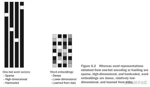
从前面的例子中也可以看到 one-hot 的这种硬编码得到的结果向量十分稀疏,并且维度比较高。
词嵌入(word embedding)是另一种将单词与向量相关联的常用方法。这种方法可以得到比 one-hot 更加密集、低维的编码。词嵌入的结果是要从数据中学习得到的。
运用词嵌入有两种方法:
利用 Embedding 层学习词嵌入:在完成着手进行的主要任务(比如文档分类或情感预测)的同时学习词嵌入:一开始使用随机的词向量,然后对词向量用与学习神经网络的权重相同的方法进行学习。
利用预训练词嵌入(pretrained word embedding):在不同于待解决问题的机器学习任务上预训练好词嵌入,然后将其加载到模型中。
利用 Embedding 层学习词嵌入
一个理想的词嵌入空间应该是可以比较完美地映射人类语言的。它是有符合现实的结构的,相近的词在空间中就应该比较接近,并且词嵌入空间中的方向也是要有意义的。例如一个比较简单的例子:
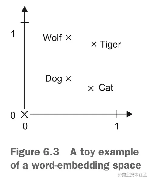
在这个词嵌入空间中,宠物都在靠下的位置,野生动物都在靠上的位置,所以一个从下到上方向的向量就应该是表示从宠物到野生动物的,这个向量从 cat 到 tiger 或者 dog -> wolf。类似的,一个从左到右的向量可以解释为从犬科到猫科,这个向量可以从 dog 到 cat,或者从 wolf 到 tiger。
再复杂一点的,比如要表示词的性别关系,将 king 向量加上 female 向量,应该得到的是 queen 向量,还有复数关系:king + plural == kings......
所以说,要有一个这样完美的词嵌入空间是很难的,现在还没有。但利用深度学习,我们还是可以得到对于特定问题来说比较好的词嵌入空间的。在 Keras 使中,我们只需要让模型学习一个 Embedding 层的权重就可以得到对当前任务的词嵌入空间:
from tensorflow.keras.layers import Embedding
embedding_layer = Embedding(1000, 64) # Embedding(可能的token个数, 嵌入的维度)
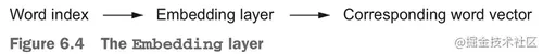
Embedding 层其实就相当于是一个字典,它将一个表示特定单词的整数索引映射到一个词向量。
Embedding 层的输入是形状为 (samples, sequence_length) 的二维整数张量。这个输入张量中的一个元素是一个代表一个文本序列的整数序列,应该保持输入的所有序列长度相同,较短的序列应该用 0 填充,较长的序列应该被截断。
Embedding 层的输出是形状为 (samples, sequence_length, embedding_dimensionality) 的三维浮点数张量。这个输出就可以用 RNN 或者 Conv1D 去处理做其他事情了。
Embedding 层一开始也是被随机初始化的,在训练过程中,会利用反向传播来逐渐调节词向量、改变空间结构,一步步接近我们之前提到的那种理想的状态。
实例:用 Embedding 层处理 IMDB 电影评论情感预测。
# 加载 IMDB 数据,准备用于 Embedding 层
from tensorflow.keras.datasets import imdb
from tensorflow.keras import preprocessing
max_features = 10000 # 作为特征的单词个数
maxlen = 20 # 在 maxlen 个特征单词后截断文本
(x_train, y_train), (x_test, y_test) = imdb.load_data(num_words=max_features)
# 将整数列表转换成形状为 (samples, maxlen) 的二维整数张量
x_train = preprocessing.sequence.pad_sequences(x_train, maxlen=maxlen)
x_test = preprocessing.sequence.pad_sequences(x_test, maxlen=maxlen)
# 在 IMDB 数据上使用 Embedding 层和分类器
from tensorflow.keras.models import Sequential
from tensorflow.keras.layers import Embedding, Flatten, Dense
model = Sequential()
model.add(Embedding(10000, 8, input_length=maxlen)) # (samples, maxlen, 8)
model.add(Flatten()) # (samles, maxlen*8)
model.add(Dense(1, activation='sigmoid')) # top classifier
model.compile(optimizer='rmsprop',
loss='binary_crossentropy',
metrics=['acc'])
model.summary()
history = model.fit(x_train, y_train,
epochs=10,
batch_size=32,
validation_split=0.2)
Model: "sequential_1"
_________________________________________________________________
Layer (type) Output Shape Param #
=================================================================
embedding_2 (Embedding) (None, 20, 8) 80000
_________________________________________________________________
flatten_1 (Flatten) (None, 160) 0
_________________________________________________________________
dense_1 (Dense) (None, 1) 161
=================================================================
Total params: 80,161
Trainable params: 80,161
Non-trainable params: 0
_________________________________________________________________
Epoch 1/10
625/625 [==============================] - 1s 1ms/step - loss: 0.6686 - acc: 0.6145 - val_loss: 0.6152 - val_acc: 0.6952
...
Epoch 10/10
625/625 [==============================] - 1s 886us/step - loss: 0.3017 - acc: 0.8766 - val_loss: 0.5260 - val_acc: 0.7508
这里我们只把词嵌入序列展开之后用一个 Dense 层去完成分类,会导致模型对输入序列中的每个词单独处理,而不去考虑单词之间的关系和句子结构。这会导致模型认为「this movie is a bomb(这电影超烂)」和「this movie is the bomb(这电影超赞)」都是负面评价。要学习句子整体的话就要用到 RNN 或者 Conv1D 了,这些之后再介绍。
使用预训练的词嵌入
和我们在做计算机视觉的时候使用预训练网络一样,在手头数据少的情况下,使用预训练的词嵌入,借用人家训练出来的可复用的模型里的通用特征。
通用的词嵌入通常是利用词频统计计算得出的,现在也有很多可供我们选用的了,比如 word2vec、GloVe 等等,具体的原理都比较复杂,我们先会用就行了。
我们会在下文的例子中尝试使用 GloVe。
从原始文本到词嵌入
我们尝试从原始的 IMDB 数据(就是一大堆文本啦)开始,处理数据,做词嵌入。
下载 IMDB 数据的原始文本
原始的 IMDB 数据集可以从 mng.bz/0tIo 下载(最后是跳转到从 aws s3下的 s3.amazonaws.com/text-datase… ,不科学上网很慢哦)。
下载的数据集解压后是这样的:
aclImdb
├── test
│ ├── neg
│ └── pos
└── train
├── neg
└── pos
在每个 neg/pos 目录下面就是一大堆 .txt 文件了,每个里面是一条评论。
下面,我们将 train 评论转换成字符串列表,一个字符串一条评论,并把对应的标签(neg/pos)写到 labels 列表。
# 处理 IMDB 原始数据的标签
import os
imdb_dir = '/Volumes/WD/Files/dataset/aclImdb'
train_dir = os.path.join(imdb_dir, 'train')
texts = []
labels = []
for label_type in ['neg', 'pos']:
dir_name = os.path.join(train_dir, label_type)
for fname in os.listdir(dir_name):
if fname.endswith('.txt'):
with open(os.path.join(dir_name, fname)) as f:
texts.append(f.read())
labels.append(0 if label_type == 'neg' else 1)
来看一下数据:
print(labels[0], texts[0], sep=' --> ')
print(labels[-1], texts[-1], sep=' --> ')
print(len(texts), len(labels))
这里 texts 和 labels 长度都是 25000。
对数据进行分词
现在来分词,顺便划分一下训练集和验证集。为了体验预训练词嵌入,我们再把训练集搞小一点,只留200条数据用来训练。
# 对 IMDB 原始数据的文本进行分词
import numpy as np
from tensorflow.keras.preprocessing.text import Tokenizer
from tensorflow.keras.preprocessing.sequence import pad_sequences
maxlen = 100 # 只看每条评论的前100个词
training_samples = 200
validation_samples = 10000
max_words = 10000
tokenizer = Tokenizer(num_words=max_words)
tokenizer.fit_on_texts(texts)
sequences = tokenizer.texts_to_sequences(texts)
word_index = tokenizer.word_index
print(f'Found {len(word_index)} unique tokens.')
data = pad_sequences(sequences, maxlen=maxlen)
labels = np.asarray(labels)
print('Shape of data tensor:', data.shape)
print('Shape of label tensor:', labels.shape)
# 打乱数据
indices = np.arange(labels.shape[0])
np.random.shuffle(indices)
data = data[indices]
labels = labels[indices]
# 划分训练、验证集
x_train = data[:training_samples]
y_train = labels[:training_samples]
x_val = data[training_samples: training_samples + validation_samples]
y_val = labels[training_samples: training_samples + validation_samples]
输出:
Found 88582 unique tokens.
Shape of data tensor: (25000, 100)
Shape of label tensor: (25000,)
下载 GloVe 词嵌入
下载预训练好的 GloVe 词嵌入: nlp.stanford.edu/data/glove.…
写下来把它解压,里面用纯文本保存了训练好的 400000 个 tokens 的 100 维词嵌入向量。
对嵌入进行预处理
解析解压后的文件:
glove_dir = '/Volumes/WD/Files/glove.6B'
embeddings_index = {}
with open(os.path.join(glove_dir, 'glove.6B.100d.txt')) as f:
for line in f:
values = line.split()
word = values[0]
coefs = np.asarray(values[1:], dtype='float32')
embeddings_index[word] = coefs
print(f'Found {len(embeddings_index)} word vectors.')
Found 400000 word vectors.
然后,我们要构建一个可以加载进 Embedding 层的嵌入矩阵,其形状为 (max_words, embedding_dim)。
embedding_dim = 100
embedding_matrix = np.zeros((max_words, embedding_dim))
for word, i in word_index.items():
if i < max_words:
embedding_vector = embeddings_index.get(word) # 有的就用 embeddings_index 里的词向量
if embedding_vector is not None: # 没有就用全零
embedding_matrix[i] = embedding_vector
print(embedding_matrix)
[[ 0. 0. 0. ... 0. 0.
0. ]
[-0.038194 -0.24487001 0.72812003 ... -0.1459 0.82779998
0.27061999]
[-0.071953 0.23127 0.023731 ... -0.71894997 0.86894
0.19539 ]
...
[-0.44036001 0.31821999 0.10778 ... -1.29849994 0.11824
0.64845002]
[ 0. 0. 0. ... 0. 0.
0. ]
[-0.54539001 -0.31817999 -0.016281 ... -0.44865 0.067047
0.17975999]]
定义模型:
from tensorflow.keras.models import Sequential
from tensorflow.keras.layers import Embedding, Flatten, Dense
model = Sequential()
model.add(Embedding(max_words, embedding_dim, input_length=maxlen))
model.add(Flatten())
model.add(Dense(32, activation='relu'))
model.add(Dense(1, activation='sigmoid'))
model.summary()
Model: "sequential_2"
_________________________________________________________________
Layer (type) Output Shape Param #
=================================================================
embedding_3 (Embedding) (None, 100, 100) 1000000
_________________________________________________________________
flatten_2 (Flatten) (None, 10000) 0
_________________________________________________________________
dense_2 (Dense) (None, 32) 320032
_________________________________________________________________
dense_3 (Dense) (None, 1) 33
=================================================================
Total params: 1,320,065
Trainable params: 1,320,065
Non-trainable params: 0
_________________________________________________________________
把 GloVe 词嵌入加载进模型
model.layers[0].set_weights([embedding_matrix])
model.layers[0].trainable = False
训练与评估模型:
model.compile(optimizer='rmsprop',
loss='binary_crossentropy',
metrics=['acc'])
history = model.fit(x_train, y_train,
epochs=10,
batch_size=32,
validation_data=(x_val, y_val))
model.save_weights('pre_trained_glove_model.h5')
绘制训练过程来看:
import matplotlib.pyplot as plt
acc = history.history['acc']
val_acc = history.history['val_acc']
loss = history.history['loss']
val_loss = history.history['val_loss']
epochs = range(len(acc))
plt.plot(epochs, acc, 'bo-', label='Training acc')
plt.plot(epochs, val_acc, 'rs-', label='Validation acc')
plt.title('Training and validation accuracy')
plt.legend()
plt.figure()
plt.plot(epochs, loss, 'bo-', label='Training loss')
plt.plot(epochs, val_loss, 'rs-', label='Validation loss')
plt.title('Training and validation loss')
plt.legend()
plt.show()
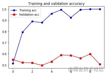
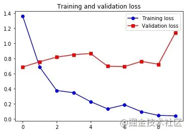
只用 200 个训练样本还是太难了,但用预训练词嵌入还是得到了不错的成果的。作为对比,看看如果不使用预训练,会是什么样的:
# 构建模型
from tensorflow.keras.models import Sequential
from tensorflow.keras.layers import Embedding, Flatten, Dense
model = Sequential()
model.add(Embedding(max_words, embedding_dim, input_length=maxlen))
model.add(Flatten())
model.add(Dense(32, activation='relu'))
model.add(Dense(1, activation='sigmoid'))
model.summary()
# 不使用 GloVe 词嵌入
# 训练
model.compile(optimizer='rmsprop',
loss='binary_crossentropy',
metrics=['acc'])
history = model.fit(x_train, y_train,
epochs=10,
batch_size=32,
validation_data=(x_val, y_val))
Model: "sequential_3"
_________________________________________________________________
Layer (type) Output Shape Param #
=================================================================
embedding_4 (Embedding) (None, 100, 100) 1000000
_________________________________________________________________
flatten_3 (Flatten) (None, 10000) 0
_________________________________________________________________
dense_4 (Dense) (None, 32) 320032
_________________________________________________________________
dense_5 (Dense) (None, 1) 33
=================================================================
Total params: 1,320,065
Trainable params: 1,320,065
Non-trainable params: 0
_________________________________________________________________
绘制训练过程:
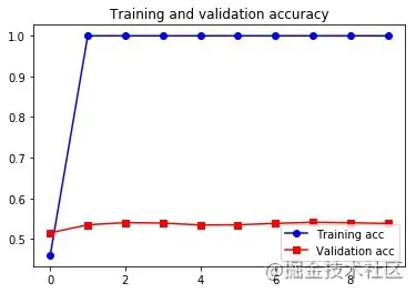
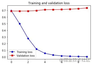
可以看到,在这个例子中,预训练词嵌入的性能要优于与任务一起学习的词嵌入。但如果有大量的可用数据,用一个 Embedding 层去与任务一起训练,通常比使用预训练词嵌入更加强大。
最后,再来看一下测试集上的结果:
# 对测试集数据进行分词
test_dir = os.path.join(imdb_dir, 'test')
texts = []
labels = []
for label_type in ['neg', 'pos']:
dir_name = os.path.join(test_dir, label_type)
for fname in sorted(os.listdir(dir_name)):
if fname.endswith('.txt'):
with open(os.path.join(dir_name, fname)) as f:
texts.append(f.read())
labels.append(0 if label_type == 'neg' else 1)
sequences = tokenizer.texts_to_sequences(texts)
x_test = pad_sequences(sequences, maxlen=maxlen)
y_test = np.asarray(labels)
# 在测试集上评估模型
model.load_weights('pre_trained_glove_model.h5')
model.evaluate(x_test, y_test)
结果:
[1.1397335529327393, 0.512719988822937]
emmm,最后的进度是令人惊讶的 50%+ !只用如此少的数据来训练还是难啊。
作者:CDFMLR
链接:https://juejin.cn/post/6993171564141215757
来源:掘金
著作权归作者所有。商业转载请联系作者获得授权,非商业转载请注明出处。
共同学习,写下你的评论
评论加载中...
作者其他优质文章