

-
.
 查看全部
查看全部 -
感知器数据分类算法步骤:
1、把权重向量W初始化为0,或把每个分量初始化为【0,1】间任意小数
2、把训练样本输入感知器,得到分类结果(-1或1)
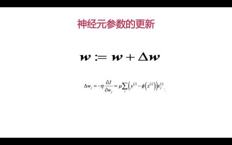
根据分类结果更新权重向量
查看全部 -
阈值的更新
查看全部 -
感知器算法试用范围
查看全部 -
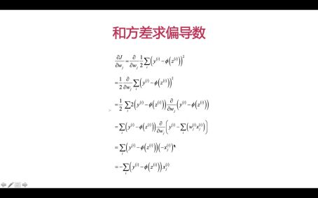
权重更新算法
查看全部 -
ada = AdalineGD(eta = 0.001, n_iter = 50)
ada.fit(x, y)
plot_decision_region(x, y, classifier = ada)
plt.title('Adaline-Gradient decent')
plt.xlabel('the length of huajing')
plt.ylabel('the length of huaban')
plt.legend(loc='upper left')
plt.show()
查看全部


举报
0/150
提交
取消