实现逻辑回归-神经网络

0|1一、基本概念

1、逻辑回归与线性回归的区别?

线性回归预测得到的是一个数值，而逻辑回归预测到的数值只有0、1两个值。逻辑回归是在线性回归的基础上，加上一个sigmoid函数，让其值位于0-1之间，最后获得的值大于0.5判断为1，小于等于0.5判断为0

0|1二、逻辑回归的推导

y^y^表示预测值，yy表示训练标签值

1、一般公式

y^=wx+by^=wx+b

2、向量化

y^=wTx+by^=wTx+b

3、激活函数
引入sigmoid函数（用σσ表示)，使y^y^值位于0-1

y^=σ(wTx+b)y^=σ(wTx+b)

4、损失函数
损失函数用LL表示

L(y^,y)=12(y^−y)2L(y^,y)=12(y^−y)2

因梯度下降效果不好，换用交叉熵损失函数

L(y^,y)=−[ylogy^+(1−y)log(1−y^)]L(y^,y)=−[ylog⁡y^+(1−y)log⁡(1−y^)]

5、代价函数
代价函数用JJ表示

J(w,b)=1m∑i=1mL(y^(i),y(i))J(w,b)=1m∑i=1mL(y^(i),y(i))

展开

J(w,b)=−1m∑i=1m[y(i)logy^(i)+(1−y(i))log(1−y^(i))]J(w,b)=−1m∑i=1m[y(i)log⁡y^(i)+(1−y(i))log⁡(1−y^(i))]

6、正向传播

a=5,b=3,c=2a=5,b=3,c=2

u=bc6u=bc6

v=a+u11v=a+u11

J=3v33J=3v33

7、反向传播

求出dada= 3，表示JJ对aa的偏导数

J=3vdJda=dJdvdvda=3J=3vdJda=dJdvdvda=3

求出dbdb= 6

J=3vdJdc=dJdvdvdududc=3c=6J=3vdJdc=dJdvdvdududc=3c=6

求出dcdc= 6

J=3vdJdb=dJdvdvdududb=3b=9J=3vdJdb=dJdvdvdududb=3b=9

对Sigmod函数求导

σ(z)=11+e−z=sσ(z)=11+e−z=s

dz=e−z(1+e−z)2dz=e−z(1+e−z)2

dz=11+e−z(1−11+e−z)dz=11+e−z(1−11+e−z)

=σ(z)(1−σ(z))=σ(z)(1−σ(z))

=s(1−s)=s(1−s)

8、反向传播的意义

修正参数，使代价函数值减少，预测值接近实际值。

举个例子：

(1) 玩一个猜数游戏，目标数字为150。

(2) 输入训练样本值: 你第一次猜出一个数字为x = 10

(3) 设置初始权重: 设置一个权重值，比如权重w设为0.5

(4) 正向计算： 进行计算，获得值wx

(5) 求出代价函数： 出题人说差了多少（说的不是具体数字，而是用0-10表示，10表示差的离谱，1表示非常接近，0表示正确）

(6) 反向传播或求导： 你通过出题人的结论，去一点点修正权重（增加w或减少w）。

(7) 重复(4)操作，直到无限接近或等于目标数字。

机器学习，就是在训练中改进、优化，找到最有泛化能力的规则。

0|1三、神经网络实现

1、实现激活函数Sigmoid

def sigmoid(z):
    s = 1.0 / (1.0 + np.exp(-z))    return s

2、参数初始化

def initialize_with_zeros(dim):
    w = np.zeros([dim,1])
    b = 0
    return w, b

3、前后向传播

def propagate(w, b, X, Y):
    m = X.shape[1]
    A = sigmoid(np.dot(w.T,X) + b)                                
    cost = (- 1.0 / m ) * np.sum(Y*np.log(A) + (1-Y)*np.log(1-A))       
    dw = (1.0 / m) * np.dot(X,(A - Y).T)
    db = (1.0 / m) * np.sum(A - Y)

    cost = np.squeeze(cost)
    grads = {"dw": dw,"db": db}    
    return grads, cost

4、优化器实现

def optimize(w, b, X, Y, num_iterations, learning_rate, print_cost = False):
    
    costs = []    
    for i in range(num_iterations):        
        # Cost and gradient calculation
        grads, cost = propagate(w,b,X,Y)        
        # Retrieve derivatives from grads
        dw = grads["dw"]
        db = grads["db"]        
        # update rule
        w = w - learning_rate * dw
        b = b - learning_rate * db        
        # Record the costs
        if i % 100 == 0:
            costs.append(cost)        
        # Print the cost every 100 training iterations
        if print_cost and i % 100 == 0:            print ("Cost after iteration %i: %f" %(i, cost))
   
    params = {"w": w,              "b": b}
    
    grads = {"dw": dw,             "db": db}    
    return params, grads, costs

5、预测函数

def predict(w, b, X):
    m = X.shape[1]
    Y_prediction = np.zeros((1,m))
    w = w.reshape(X.shape[0], 1)    # Compute vector "A" predicting the probabilities of a cat being present in the picture
    A = sigmoid(np.dot(w.T,X)+b)    for i in range(A.shape[1]):        # Convert probabilities A[0,i] to actual predictions p[0,i]
        if A[0][i] <= 0.5:
            Y_prediction[0][i] = 0
        else:
            Y_prediction[0][i] = 1

    return Y_prediction

6、代码模块整合

def model(X_train, Y_train, X_test, Y_test, num_iterations = 2000, learning_rate = 0.5, print_cost = False):

    # initialize parameters with zeros (≈ 1 line of code)
    w, b = initialize_with_zeros(train_set_x.shape[0])    # Gradient descent (≈ 1 line of code)
    parameters, grads, costs = optimize(w, b, X_train, Y_train, num_iterations, learning_rate, print_cost)    
    # Retrieve parameters w and b from dictionary "parameters"
    w = parameters["w"]
    b = parameters["b"]
    
    Y_prediction_test = predict(w, b, X_test)
    Y_prediction_train = predict(w, b, X_train)    # Print train/test Errors
    print("train accuracy: {} %".format(100 - np.mean(np.abs(Y_prediction_train - Y_train)) * 100))
    print("test accuracy: {} %".format(100 - np.mean(np.abs(Y_prediction_test - Y_test)) * 100))

    
    d = {"costs": costs,         "Y_prediction_test": Y_prediction_test, 
         "Y_prediction_train" : Y_prediction_train, 
         "w" : w, 
         "b" : b,         "learning_rate" : learning_rate,         "num_iterations": num_iterations}    
    return d

7、运行程序

d = model(train_set_x, train_set_y, test_set_x, test_set_y, num_iterations = 2000, learning_rate = 0.005, print_cost = True)

结果

Cost after iteration 0: 0.693147Cost after iteration 100: 0.584508Cost after iteration 200: 0.466949Cost after iteration 300: 0.376007Cost after iteration 400: 0.331463Cost after iteration 500: 0.303273Cost after iteration 600: 0.279880Cost after iteration 700: 0.260042Cost after iteration 800: 0.242941Cost after iteration 900: 0.228004Cost after iteration 1000: 0.214820Cost after iteration 1100: 0.203078Cost after iteration 1200: 0.192544Cost after iteration 1300: 0.183033Cost after iteration 1400: 0.174399Cost after iteration 1500: 0.166521Cost after iteration 1600: 0.159305Cost after iteration 1700: 0.152667Cost after iteration 1800: 0.146542Cost after iteration 1900: 0.140872train accuracy: 99.04306220095694 %test accuracy: 70.0 %

8、更多的分析

learning_rates = [0.01, 0.001, 0.0001]
models = {}for i in learning_rates:    print ("learning rate is: " + str(i))
    models[str(i)] = model(train_set_x, train_set_y, test_set_x, test_set_y, num_iterations = 1500, learning_rate = i, print_cost = False)    print ('\n' + "-------------------------------------------------------" + '\n')for i in learning_rates:
    plt.plot(np.squeeze(models[str(i)]["costs"]), label= str(models[str(i)]["learning_rate"]))

plt.ylabel('cost')
plt.xlabel('iterations (hundreds)')

legend = plt.legend(loc='upper center', shadow=True)
frame = legend.get_frame()
frame.set_facecolor('0.90')
plt.show()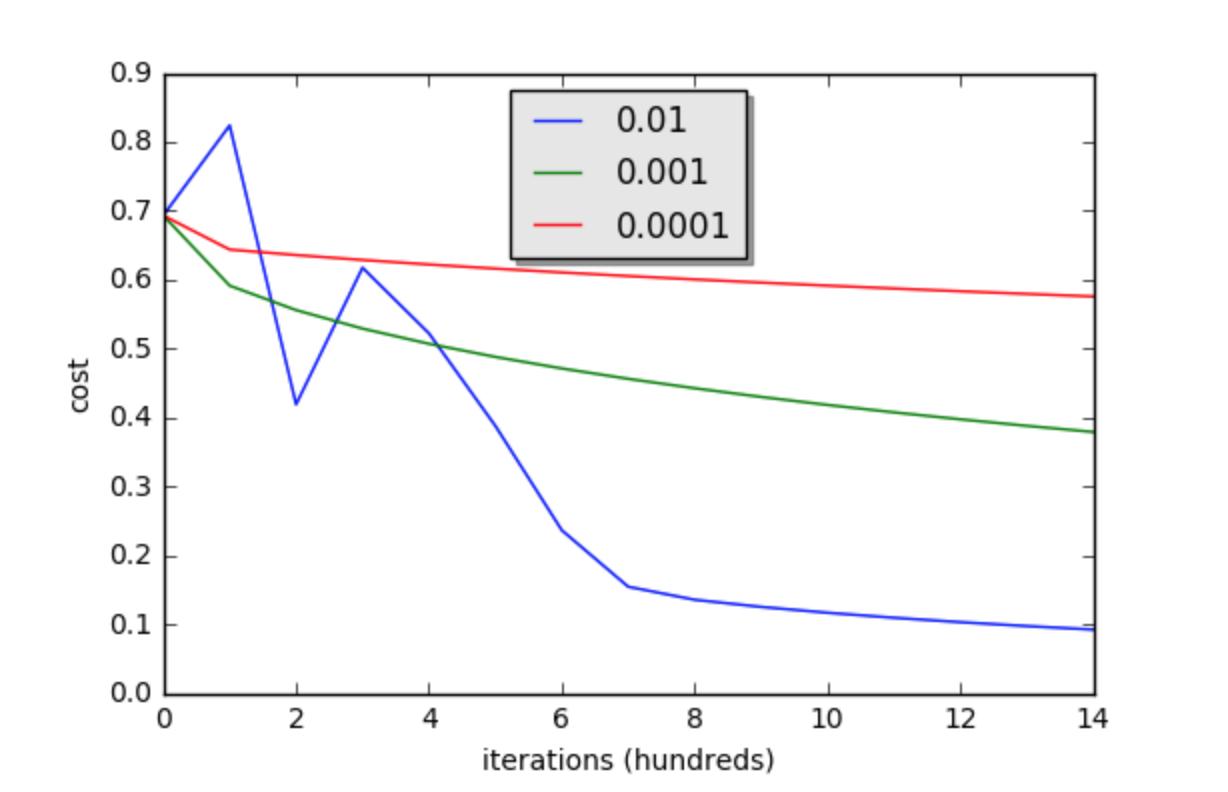

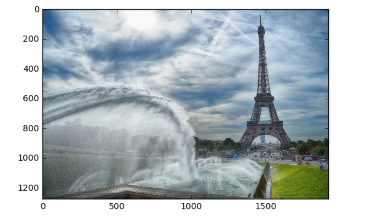
9、测试图片

## START CODE HERE ## (PUT YOUR IMAGE NAME) my_image = "my_image.jpg"   # change this to the name of your image file ## END CODE HERE ### We preprocess the image to fit your algorithm.fname = "images/" + my_image
image = np.array(ndimage.imread(fname, flatten=False))
my_image = scipy.misc.imresize(image, size=(num_px,num_px)).reshape((1, num_px*num_px*3)).T
my_predicted_image = predict(d["w"], d["b"], my_image)

plt.imshow(image)
print("y = " + str(np.squeeze(my_predicted_image)) + ", your algorithm predicts a \"" + classes[int(np.squeeze(my_predicted_image)),].decode("utf-8") +  "\" picture.")

结果

y = 0.0, your algorithm predicts a "non-cat" picture.

参考文档

神经网络和深度学习-吴恩达——Course1 Week2

__EOF__

作　　者：fonxian
出　　处：https://www.cnblogs.com/fonxian/p/10459762.html