
在本系列的前文 [1,2]中,我们介绍了如何使用 Python 语言图分析库 NetworkX [3] + Nebula Graph [4] 来进行<权力的游戏>中人物关系图谱分析。
在本文中我们将介绍如何使用 Java 语言的图分析库 JGraphT [5] 并借助绘图库 mxgraph [6] ,可视化探索 A 股的行业个股的相关性随时间的变化情况。

数据集的处理
本文主要分析方法参考了[7,8],有两种数据集:
股票数据(点集)
从 A 股中按股票代码顺序选取了 160 只股票(排除摘牌或者 ST 的)。每一支股票都被建模成一个点,每个点的属性有股票代码,股票名称,以及证监会对该股票对应上市公司所属板块分类等三种属性;
表1:点集示例
| 顶点id | 股票代码 | 股票名称 | 所属板块 |
|---|---|---|---|
| 1 | SZ0001 | 平安银行 | 金融行业 |
| 2 | 600000 | 浦发银行 | 金融行业 |
| 3 | 600004 | 白云机场 | 交通运输 |
| 4 | 600006 | 东风汽车 | 汽车制造 |
| 5 | 600007 | 中国国贸 | 开发区 |
| 6 | 600008 | 首创股份 | 环保行业 |
| 7 | 600009 | 上海机场 | 交通运输 |
| 8 | 600010 | 包钢股份 | 钢铁行业 |
股票关系(边集)
边只有一个属性,即权重。边的权重代表边的源点和目标点所代表的两支股票所属上市公司业务上的的相似度——相似度的具体计算方法参考 [7,8]:取一段时间(2014 年 1 月 1 日 - 2020 年 1 月 1 日)内,个股的日收益率的时间序列相关性  再定义个股之间的距离为 (也即两点之间的边权重):
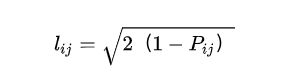
通过这样的处理,距离取值范围为 [0,2]。这意味着距离越远的个股,两个之间的收益率相关性越低。
表2: 边集示例
| 边的源点 ID | 边的目标点 ID | 边的权重 |
|---|---|---|
| 11 | 12 | 0.493257968 |
| 22 | 83 | 0.517027513 |
| 23 | 78 | 0.606206233 |
| 2 | 12 | 0.653692415 |
| 1 | 11 | 0.677631482 |
| 1 | 27 | 0.695705171 |
| 1 | 12 | 0.71124344 |
| 2 | 11 | 0.73581915 |
| 8 | 18 | 0.771556458 |
| 12 | 27 | 0.785046446 |
| 9 | 20 | 0.789606527 |
| 11 | 27 | 0.796009627 |
| 25 | 63 | 0.797218349 |
| 25 | 72 | 0.799230001 |
| 63 | 115 | 0.803534952 |
这样的点集和边集构成一个图网络,可以将这个网络存储在图数据库 Nebula Graph 中。
JGraphT
JGraphT 是一个开放源代码的 Java 类库,它不仅为我们提供了各种高效且通用的图数据结构,还为解决最常见的图问题提供了许多有用的算法:
-
支持有向边、无向边、权重边、非权重边等;
-
支持简单图、多重图、伪图;
-
提供了用于图遍历的专用迭代器(DFS,BFS)等;
-
提供了大量常用的的图算法,如路径查找、同构检测、着色、公共祖先、游走、连通性、匹配、循环检测、分区、切割、流、中心性等算法;
-
可以方便地导入 / 导出 GraphViz [9]。导出的 GraphViz 可被导入可视化工具 Gephi[10] 进行分析与展示;
-
可以方便地使用其他绘图组件,如:JGraphX,mxGraph,Guava Graphs Generators 等工具绘制出图网络。
下面,我们来实践一把,先在 JGraphT 中创建一个有向图:
import org.jgrapht.*;

import org.jgrapht.graph.*;

import org.jgrapht.nio.*;

import org.jgrapht.nio.dot.*;

import org.jgrapht.traverse.*;


import java.io.*;

import java.net.*;

import java.util.*;


Graph<URI, DefaultEdge> g = new  DefaultDirectedGraph<>(DefaultEdge.class);
添加顶点:
URI  google = new  URI("http://www.google.com");

URI  wikipedia = new  URI("http://www.wikipedia.org");

URI  jgrapht = new  URI("http://www.jgrapht.org");


// add the vertices

g.addVertex(google);

g.addVertex(wikipedia);

g.addVertex(jgrapht);
添加边:
// add edges to create linking structure

g.addEdge(jgrapht, wikipedia);

g.addEdge(google, jgrapht);

g.addEdge(google, wikipedia);

g.addEdge(wikipedia, google);
图数据库 Nebula Graph Database
JGraphT 通常使用本地文件作为数据源,这在静态网络研究的时候没什么问题,但如果图网络经常会发生变化——例如,股票数据每日都在变化——每次生成全新的静态文件再加载分析就有些麻烦,最好整个变化过程可以持久化地写入一个数据库中,并且可以实时地直接从数据库中加载子图或者全图做分析。本文选用 Nebula Graph 作为存储图数据的图数据库。
Nebula Graph 的 Java 客户端 Nebula-Java [11] 提供了两种访问 Nebula Graph 方式:一种是通过图查询语言 nGQL [12] 与查询引擎层 [13] 交互,这通常适用于有复杂语义的子图访问类型; 另一种是通过 API 与底层的存储层(storaged)[14] 直接交互,用于获取全量的点和边。除了可以访问 Nebula Graph 本身外,Nebula-Java 还提供了与 Neo4j [15]、JanusGraph [16]、Spark [17] 等交互的示例。
在本文中,我们选择直接访问存储层(storaged)来获取全部的点和边。下面两个接口可以用来读取所有的点、边数据:
// space 为待扫描的图空间名称,returnCols 为需要读取的点/边及其属性列,

// returnCols 参数格式:{tag1Name: prop1, prop2, tag2Name: prop3, prop4, prop5}

Iterator<ScanVertexResponse> scanVertex(

String space, Map<String, List<String>> returnCols);

Iterator<ScanEdgeResponse> scanEdge(

String space, Map<String, List<String>> returnCols);
第一步:初始化一个客户端,和一个 ScanVertexProcessor。ScanVertexProcessor 用来对读出来的顶点数据进行解码:
MetaClientImpl  metaClientImpl = new  MetaClientImpl(metaHost, metaPort);

metaClientImpl.connect();

StorageClient  storageClient = new  StorageClientImpl(metaClientImpl);

Processor  processor = new  ScanVertexProcessor(metaClientImpl);
第二步:调用 scanVertex 接口,该接口会返回一个 scanVertexResponse 对象的迭代器:
Iterator<ScanVertexResponse> iterator =

storageClient.scanVertex(spaceName, returnCols);
第三步:不断读取该迭代器所指向的 scanVertexResponse 对象中的数据,直到读取完所有数据。读取出来的顶点数据先保存起来,后面会将其添加到到 JGraphT 的图结构中:
while (iterator.hasNext()) {

ScanVertexResponse  response = iterator.next();

if (response == null) {

log.error("Error occurs while scan vertex");

break;

}

Result  result = processor.process(spaceName, response);

results.addAll(result.getRows(TAGNAME));

}
读取边数据的方法和上面的流程类似。
在 JGraphT 中进行图分析
第一步:在 JGraphT 中创建一个无向加权图 graph:
Graph<String, MyEdge> graph = GraphTypeBuilder

.undirected()

.weighted(true)

.allowingMultipleEdges(true)

.allowingSelfLoops(false)

.vertexSupplier(SupplierUtil.createStringSupplier())

.edgeSupplier(SupplierUtil.createSupplier(MyEdge.class))

.buildGraph();
第二步:将上一步从 Nebula Graph 图空间中读出来的点、边数据添加到 graph 中:
for (VertexDomain  vertex  : vertexDomainList){

graph.addVertex(vertex.getVid().toString());

stockIdToName.put(vertex.getVid().toString(), vertex);

}


for (EdgeDomain  edgeDomain  : edgeDomainList){

graph.addEdge(edgeDomain.getSrcid().toString(), edgeDomain.getDstid().toString());

MyEdge  newEdge = graph.getEdge(edgeDomain.getSrcid().toString(), edgeDomain.getDstid().toString());

graph.setEdgeWeight(newEdge, edgeDomain.getWeight());

}
第三步:参考 [7,8] 中的分析法,对刚才的图 graph 使用 Prim 最小生成树算法(minimun-spanning-tree),并调用封装好的 drawGraph 接口画图:
普里姆算法(Prim’s algorithm),图论中的一种算法,可在加权连通图里搜索最小生成树。即,由此算法搜索到的边子集所构成的树中,不但包括了连通图里的所有顶点,且其所有边的权值之和亦为最小。
SpanningTreeAlgorithm.SpanningTree  pMST = new  PrimMinimumSpanningTree(graph).getSpanningTree();


Legend.drawGraph(pMST.getEdges(), filename, stockIdToName);
第四步:drawGraph 方法封装了画图的布局等各项参数设置。这个方法将同一板块的股票渲染为同一颜色,将距离接近的股票排列聚集在一起。
public  class  Legend {

...

public  static  void  drawGraph(Set<MyEdge> edges, String  filename, Map<String, VertexDomain> idVertexMap) throws  IOException {

// Creates graph with model

mxGraph graph = new mxGraph();

Object  parent = graph.getDefaultParent();


// set style

graph.getModel().beginUpdate();

mxStylesheet myStylesheet = graph.getStylesheet();

graph.setStylesheet(setMsStylesheet(myStylesheet));


Map<String, Object> idMap = new  HashMap<>();

Map<String, String> industryColor = new  HashMap<>();


int  colorIndex = 0;


for (MyEdge  edge  : edges) {

Object  src, dst;

if (!idMap.containsKey(edge.getSrc())) {

VertexDomain  srcNode = idVertexMap.get(edge.getSrc());

String  nodeColor;

if (industryColor.containsKey(srcNode.getIndustry())){

nodeColor = industryColor.get(srcNode.getIndustry());

}else {

nodeColor = COLOR_LIST[colorIndex++];

industryColor.put(srcNode.getIndustry(), nodeColor);

}

src = graph.insertVertex(parent, null, srcNode.getName(), 0, 0, 105, 50, "fillColor=" + nodeColor);

idMap.put(edge.getSrc(), src);

} else {

src = idMap.get(edge.getSrc());

}


if (!idMap.containsKey(edge.getDst())) {

VertexDomain  dstNode = idVertexMap.get(edge.getDst());


String  nodeColor;

if (industryColor.containsKey(dstNode.getIndustry())){

nodeColor = industryColor.get(dstNode.getIndustry());

}else {

nodeColor = COLOR_LIST[colorIndex++];

industryColor.put(dstNode.getIndustry(), nodeColor);

}


dst = graph.insertVertex(parent, null, dstNode.getName(), 0, 0, 105, 50, "fillColor=" + nodeColor);

idMap.put(edge.getDst(), dst);

} else {

dst = idMap.get(edge.getDst());

}

graph.insertEdge(parent, null, "", src, dst);

}


log.info("vertice " + idMap.size());

log.info("colorsize " + industryColor.size());


mxFastOrganicLayout layout = new mxFastOrganicLayout(graph);

layout.setMaxIterations(2000);

//layout.setMinDistanceLimit(10D);

layout.execute(parent);


graph.getModel().endUpdate();


// Creates an image than can be saved using ImageIO

BufferedImage  image = createBufferedImage(graph, null, 1, Color.WHITE,

true, null);


// For the sake of this example we display the image in a window

// Save as JPEG

File  file = new  File(filename);

ImageIO.write(image, "JPEG", file);


}

...

}
第五步:生成可视化:
图1中每个顶点的颜色代表证监会对该股票所属上市公司归类的板块。
可以看到,实际业务近似度较高的股票已经聚拢成簇状(例如:高速板块、银行版本、机场航空板块),但也会有部分关联性不明显的个股被聚类在一起,具体原因需要单独进行个股研究。

图1: 基于 2015-01-01 至 2020-01-01 的股票数据计算出的聚集性
第六步:基于不同时间窗口的一些其他动态探索
上节中,结论主要基于 2015-01-01 到 2020-01-01 的个股聚集性。这一节我们还做了一些其他的尝试:以 2 年为一个时间滑动窗口,分析方法不变,定性探索聚集群是否随着时间变化会发生改变。

图2:基于 2014-01-01 至 2016-01-01 的股票数据计算出的聚集性

图3:基于 2015-01-01 至 2017-01-01 的股票数据计算出的聚集性

图4:基于 2016-01-01 至 2018-01-01 的股票数据计算出的聚集性

图5:基于 2017-01-01 至 2019-01-01 的股票数据计算出的聚集性

图6:基于 2018-01-01 至 2020-01-01 的股票数据计算出的聚集性
粗略分析看,随着时间窗口变化,有些板块(高速、银行、机场航空、房产、能源)的板块内部个股聚集性一直保持比较好——这意味着随着时间变化,这个版块内各种一直保持比较高的相关性;但有些板块(制造)的聚集性会持续变化——意味着相关性一直在发生变化。
Disclaim

本文不构成任何投资建议,且作者不持有本文中任一股票。
受限于停牌、熔断、涨跌停、送转、并购、主营业务变更等情况,数据处理可能有错误,未做一一检查。
受时间所限,本文只选用了 160 个个股样本过去 6 年的数据,只采用了最小扩张树一种办法来做聚类分类。未来可以使用更大的数据集(例如美股、衍生品、数字货币),尝试更多种图机器学习的办法。
本文代码可见[18]
Reference
[1] 用 NetworkX + Gephi + Nebula Graph 分析<权力的游戏>人物关系(上篇)https://nebula-graph.com.cn/posts/game-of-thrones-relationship-networkx-gephi-nebula-graph/
[2] 用 NetworkX + Gephi + Nebula Graph 分析<权力的游戏>人物关系(下篇) https://nebula-graph.com.cn/posts/game-of-thrones-relationship-networkx-gephi-nebula-graph-part-two/
[3] NetworkX: a Python package for the creation, manipulation, and study of the structure, dynamics, and functions of complex networks. https://networkx.github.io/
[4] Nebula Graph: A powerfully distributed, scalable, lightning-fast graph database written in C++. https://nebula-graph.io/
[5] JGraphT: a Java library of graph theory data structures and algorithms. https://jgrapht.org/
[6] mxGraph: JavaScript diagramming library that enables interactive graph and charting applications. https://jgraph.github.io/mxgraph/
[7] Bonanno, Giovanni & Lillo, Fabrizio & Mantegna, Rosario. (2000). High-frequency Cross-correlation in a Set of Stocks. arXiv.org, Quantitative Finance Papers. 1. 10.1080/713665554.
[8] Mantegna, R.N. Hierarchical structure in financial markets. Eur. Phys. J. B 11, 193–197 (1999).
[10] https://gephi.org/
[12] Nebula Graph Query Language (nGQL). https://docs.nebula-graph.io/manual-EN/1.overview/1.concepts/2.nGQL-overview/
[13] Nebula Graph Query Engine. https://github.com/vesoft-inc/nebula-graph
[14] Nebula-storage: A distributed consistent graph storage. https://github.com/vesoft-inc/nebula-storage
[15] Neo4j. www.neo4j.com
[16] JanusGraph. janusgraph.org
[17] Apache Spark. spark.apache.org.
共同学习,写下你的评论
评论加载中...
作者其他优质文章