[Python人工智能] 五.theano实现神经网络正规化Regularization处理

一. 正规化-Regularization

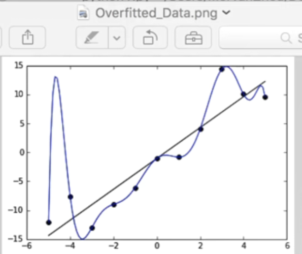
在用神经网络分析数据时，通常会遇到Overfitting问题。如下图所示，分布了很多黑色的数据点，如果机器学习能学到一条黑色直线去代替我们分布的数据散点，并预测我们的数据分布，那这条直线就是学习得到的一条很好的线条。

但是Overfitting会产生一个问题：在学习过程中会不断减小与真实值的误差，得到这条蓝色的线条，它能非常完美的预测这些点，与真实值的误差非常小，误差cost甚至为0，而黑色的直线的会与真实值产生误差。例如，x为-4这个点，蓝色线对应值为-7，基本吻合，而黑色线预测值为-12，存在一定误差。

但真实预测时，我们会觉得黑色线比蓝色线更为准确，因为如果有其他数据点时，将来的数据用黑色的线能更好的进行预测或概括。比如x为2.5时，蓝色线这个点的误差可能会比黑色线更大。Overfitting后的误差会非常小，但是测试数据时误差会突然变得很大，并且没有黑线预测的结果好。

这就是回归中Overfitting的一种形式 ，那么如果是分类问题，Overfitting又怎么体现呢？
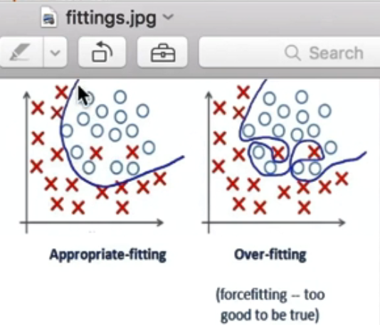
分类问题，看下面这张图。第一张图通过一条曲线将data分割开来，注意有两个X在class2里面；第二张图是Over-fitting完全把数据点分离开来，一堆点为class1、另一堆点为class2。虽然训练时图2误差更小，但是使用图2去预测时，其误差可能会更大，而图1的误差会更小，更倾向于用图1的方法。

避免Over-fitting的方法主要是正规化，包括Regularization L1和L2，下面开始讲解。

二. 定义Layer类及增加数据集

1.定义Layer类

神经网络首先需要添加神经层，将层（Layer）定义成类，通过类来添加神经层。神经层是相互链接，并且是全连接，从第一层输入层传入到隐藏层，最后传输至输出层。假设接下来需要定义两层内容：
    L1 = Layer(inputs, in_size=13, out_size=50, activation_function)
    参数包括输入值，输入节点数，输出节点数和激励函数
    L2 = Layer(L1.outputs, 50, 1, None)
    参数中L1的输出作为输入值，L1的输出10个节点作为输入节点，输出节点1个，激励函数为None。

定义类的代码如下，包括权重和bias，其中参数为随机变量更有利于我们后面的更新，乱序更能促进神经网络的学习。

1. #coding:utf-8  

2. import numpy as np  

3. import theano.tensor as T  

4. import theano  

5. from theano import function  

6. from sklearn.datasets import load_boston  

7. import matplotlib.pyplot as plt  

8.   

9. #首先定义神经网络Layer类  

10. class Layer(object):  

11.     def __init__(self, inputs, in_size, out_size, activation_function=None):  

12.         #权重: 平均值为0 方差为1 行数为in_size  列数为out_size  

13.         self.W = theano.shared(np.random.normal(0,1,(in_size,out_size)))  

14.         #bias  

15.         self.b = theano.shared(np.zeros((out_size,) ) + 0.1)  

16.         #乘法加bias  

17.         self.Wx_plus_b = T.dot(inputs, self.W) + self.b #dot乘法  

18.         #激励函数  

19.         self.activation_function = activation_function  

20.   

21.         #默认为None,否则进行激活  

22.         if activation_function is None:   

23.             self.outputs = self.Wx_plus_b  

24.         else:   

25.             self.outputs = self.activation_function(self.Wx_plus_b)  

2.增加数据集

需要注意，机器学习通常将数据data划分为两组，train data-训练神经网络、test data-检验预测神经网络。这里所采用的数据集是sklearn中的波士顿房价数据集（load_boston），该数据集包括500多个数据点，每个sample有13个特征去描述房价。

再导入数据集之前，作者补充一个知识点——Nnormalization。

通过 "x_data = load_boston().data" 代码导入波士顿房价数据集，但是x_data变化范围非常之广，比如有一个特征是占地面积，其范围从0到500，而另一个特征到市中心的距离，值为1、2公里，由于0到500和0到2取值范围变化幅度较大，这里使用机器学习机器一种技巧 Normalization 进行处理。将x的特征进行正常化，把每个特征的取值范围都浓缩到0-1的范围，这样能使机器学习更方便的学习东西，这里我主要通过自定义函数minmax_normalization()实现。代码如下：

1. #coding:utf-8  

2. import numpy as np  

3. import theano.tensor as T  

4. import theano  

5. from theano import function  

6. from sklearn.datasets import load_boston  

7. import matplotlib.pyplot as plt  

8.   

9. #首先定义神经网络Layer类  

10. class Layer(object):  

11.     def __init__(self, inputs, in_size, out_size, activation_function=None):  

12.         #权重: 平均值为0 方差为1 行数为in_size  列数为out_size  

13.         self.W = theano.shared(np.random.normal(0,1,(in_size,out_size)))  

14.         #bias  

15.         self.b = theano.shared(np.zeros((out_size,) ) + 0.1)  

16.         #乘法加bias  

17.         self.Wx_plus_b = T.dot(inputs, self.W) + self.b #dot乘法  

18.         #激励函数  

19.         self.activation_function = activation_function  

20.   

21.         #默认为None,否则进行激活  

22.         if activation_function is None:   

23.             self.outputs = self.Wx_plus_b  

24.         else:   

25.             self.outputs = self.activation_function(self.Wx_plus_b)  

26.   

27. #正常化处理 数据降为0-1之间  

28. def minmax_normalization(data):  

29.     xs_max = np.max(data, axis=0)  

30.     xs_min = np.min(data, axis=0)  

31.     xs = (1-0) * (data - xs_min) / (xs_max - xs_min) + 0  

32.     return xs   

33.   

34. #导入sklearn中的波士顿房价数据集  

35. #500多个数据点 每个sample有13个特征去描述房价  

36. np.random.seed(100)  

37. x_data = load_boston().data #数据集  

38.   

39. #minmax normalization, rescale the inputs  

40. x_data = minmax_normalization(x_data)  

41. print(x_data)  

42. #增加一个维度 定义成矩阵的形式  

43. y_data = load_boston().target[:, np.newaxis]   

44. print(y_data)  

45.   

46. #cross validation, train test data split  

47. #划分训练集和测试集  

48. #前400个sameple或样本行作为训练集, 剩余的作为预测集  

49. x_train, y_train = x_data[:400], y_data[:400]  

50. x_test, y_test = x_data[400:], y_data[400:]  

51. print(x_train.shape, y_train.shape)  

52. print(x_test.shape, y_test.shape)  

输出结果如下图所示，包括13个特征Normalization后的结果，y类标及划分为训练集和预测集的形状。

1. [[0.00000000e+00 1.80000000e-01 6.78152493e-02 ... 2.87234043e-01  

2.   1.00000000e+00 8.96799117e-02]  

3.  [2.35922539e-04 0.00000000e+00 2.42302053e-01 ... 5.53191489e-01  

4.   1.00000000e+00 2.04470199e-01]  

5.  [2.35697744e-04 0.00000000e+00 2.42302053e-01 ... 5.53191489e-01  

6.   9.89737254e-01 6.34657837e-02]  

7.  ...  

8.  [6.11892474e-04 0.00000000e+00 4.20454545e-01 ... 8.93617021e-01  

9.   1.00000000e+00 1.07891832e-01]  

10.  [1.16072990e-03 0.00000000e+00 4.20454545e-01 ... 8.93617021e-01  

11.   9.91300620e-01 1.31070640e-01]  

12.  [4.61841693e-04 0.00000000e+00 4.20454545e-01 ... 8.93617021e-01  

13.   1.00000000e+00 1.69701987e-01]]  

14. [[24. ]  

15.  [21.6]  

16.  [34.7]  

17.  [33.4]  

18.  [36.2]  

19.  ...  

20.  [16.8]  

21.  [22.4]  

22.  [20.6]  

23.  [23.9]  

24.  [22. ]  

25.  [11.9]]  

26. (400, 13) (400, 1)  

27. (106, 13) (106, 1)  

三. theano实现回归神经网络正规化

1.定义变量和Layer

包括两个Layer，如下：
L1: 13个属性，神经层有50个神经元，激活函数用tanh
    L1 = Layer(x, 13, 50, T.tanh)
L2: 输入为L1输出，输入个数为50，输出为1即房价
    L2 = Layer(L1.outputs, 50, 1, None)

1. #coding:utf-8  

2. import numpy as np  

3. import theano.tensor as T  

4. import theano  

5. from theano import function  

6. from sklearn.datasets import load_boston  

7. import matplotlib.pyplot as plt  

8.   

9. #首先定义神经网络Layer类  

10. class Layer(object):  

11.     def __init__(self, inputs, in_size, out_size, activation_function=None):  

12.         #权重: 平均值为0 方差为1 行数为in_size  列数为out_size  

13.         self.W = theano.shared(np.random.normal(0,1,(in_size,out_size)))  

14.         #bias  

15.         self.b = theano.shared(np.zeros((out_size,) ) + 0.1)  

16.         #乘法加bias  

17.         self.Wx_plus_b = T.dot(inputs, self.W) + self.b #dot乘法  

18.         #激励函数  

19.         self.activation_function = activation_function  

20.   

21.         #默认为None,否则进行激活  

22.         if activation_function is None:   

23.             self.outputs = self.Wx_plus_b  

24.         else:   

25.             self.outputs = self.activation_function(self.Wx_plus_b)  

26.   

27. #正常化处理 数据降为0-1之间  

28. def minmax_normalization(data):  

29.     xs_max = np.max(data, axis=0)  

30.     xs_min = np.min(data, axis=0)  

31.     xs = (1-0) * (data - xs_min) / (xs_max - xs_min) + 0  

32.     return xs   

33.   

34. #导入sklearn中的波士顿房价数据集  

35. #500多个数据点 每个sample有13个特征去描述房价  

36. np.random.seed(100)  

37. x_data = load_boston().data #数据集  

38.   

39. #minmax normalization, rescale the inputs  

40. x_data = minmax_normalization(x_data)  

41. print(x_data)  

42. #增加一个维度 定义成矩阵的形式  

43. y_data = load_boston().target[:, np.newaxis]   

44. print(y_data)  

45.   

46. #cross validation, train test data split  

47. #划分训练集和测试集  

48. #前400个sameple或样本行作为训练集, 剩余的作为预测集  

49. x_train, y_train = x_data[:400], y_data[:400]  

50. x_test, y_test = x_data[400:], y_data[400:]  

51. print(x_train.shape, y_train.shape)  

52. print(x_test.shape, y_test.shape)  

53.   

54.   

55. #定义x和y  

56. x = T.dmatrix("x")  

57. y = T.dmatrix("y")  

58.   

59. #定义两个Layer  

60. #L1: 13个属性，神经层有50个神经元，激活函数用tanh  

61. L1 = Layer(x, 13, 50, T.tanh)  

62. #L2: 输入为L1输出，输入个数为50，输出为1即房价  

63. L2 = Layer(L1.outputs, 50, 1, None)  

2.计算误差

（1）普通方法
定义cost变量计算误差，即预测值与真实值的差别。常用的方法如下，通过计算输出结果（预测值）和真实结果误差的平方平均自实现。
    cost = T.mean(T.square(L2.outputs-y))
但是该方法会产生Overfitting问题。为了解决Overfitting，在计算cost时，我要做一些手脚，加上一个东西。

（2）L2 Regularization
    cost = T.mean(T.square(L2.outputs-y)) + 0.1*((L1.W**2).sum() + (L2.W**2).sum())
它是0.1乘以L1的权重平方求和加上L2的权重平方和，注意尽量用一个小于1的值来乘，如这里的0.1。
上面这个就是L2 Regularization方法，相当于有一个 0.1乘以所有的weight平方和，它称为惩罚机制。快要进入Overfitting时，通过这个机制来惩罚，不进入Overfitting，另一种方法是L1 Regularization。

（3）L1 Regularization
    cost = T.mean(T.square(L2.outputs-y)) + 0.1*(abs(L1.W).sum() + abs(L2.W).sum())
根据流行程度来看，L2比L1更普及，这篇文章也主要使用L2进行实验，0.1可以取不同值，去分别测试对比实验。

1. #coding:utf-8  

2. import numpy as np  

3. import theano.tensor as T  

4. import theano  

5. from theano import function  

6. from sklearn.datasets import load_boston  

7. import matplotlib.pyplot as plt  

8.   

9. #首先定义神经网络Layer类  

10. class Layer(object):  

11.     def __init__(self, inputs, in_size, out_size, activation_function=None):  

12.         #权重: 平均值为0 方差为1 行数为in_size  列数为out_size  

13.         self.W = theano.shared(np.random.normal(0,1,(in_size,out_size)))  

14.         #bias  

15.         self.b = theano.shared(np.zeros((out_size,) ) + 0.1)  

16.         #乘法加bias  

17.         self.Wx_plus_b = T.dot(inputs, self.W) + self.b #dot乘法  

18.         #激励函数  

19.         self.activation_function = activation_function  

20.   

21.         #默认为None,否则进行激活  

22.         if activation_function is None:   

23.             self.outputs = self.Wx_plus_b  

24.         else:   

25.             self.outputs = self.activation_function(self.Wx_plus_b)  

26.   

27. #正常化处理 数据降为0-1之间  

28. def minmax_normalization(data):  

29.     xs_max = np.max(data, axis=0)  

30.     xs_min = np.min(data, axis=0)  

31.     xs = (1-0) * (data - xs_min) / (xs_max - xs_min) + 0  

32.     return xs   

33.   

34. #导入sklearn中的波士顿房价数据集  

35. #500多个数据点 每个sample有13个特征去描述房价  

36. np.random.seed(100)  

37. x_data = load_boston().data #数据集  

38.   

39. #minmax normalization, rescale the inputs  

40. x_data = minmax_normalization(x_data)  

41. print(x_data)  

42. #增加一个维度 定义成矩阵的形式  

43. y_data = load_boston().target[:, np.newaxis]   

44. print(y_data)  

45.   

46. #cross validation, train test data split  

47. #划分训练集和测试集  

48. #前400个sameple或样本行作为训练集, 剩余的作为预测集  

49. x_train, y_train = x_data[:400], y_data[:400]  

50. x_test, y_test = x_data[400:], y_data[400:]  

51. print(x_train.shape, y_train.shape)  

52. print(x_test.shape, y_test.shape)  

53.   

54.   

55. #定义x和y  

56. x = T.dmatrix("x")  

57. y = T.dmatrix("y")  

58.   

59. #定义两个Layer  

60. #L1: 13个属性，神经层有50个神经元，激活函数用tanh  

61. L1 = Layer(x, 13, 50, T.tanh)  

62. #L2: 输入为L1输出，输入个数为50，输出为1即房价  

63. L2 = Layer(L1.outputs, 50, 1, None)  

64.   

65.   

66. #the way to compute cost  

67. #计算误差 但该方法的结果会产生Overfitting问题  

68. cost = T.mean(T.square(L2.outputs-y))  

69.   

70. #L2 regularization  

71. #0.1乘以L1的权重平方求和加上L2的权重平方和  

72. #惩罚机制: 快要进入Overfitting时，通过这个机制来惩罚不进入Overfitting  

73. cost = T.mean(T.square(L2.outputs-y)) + 0.1*((L1.W**2).sum() + (L2.W**2).sum())  

74.   

75. #L1 regularization  

76. cost = T.mean(T.square(L2.outputs-y)) + 0.1*(abs(L1.W).sum() + abs(L2.W).sum())  

3.梯度下降更新

再定义梯度下降变量，其误差越大，降低趋势越大，通过梯度下降让预测值更接近真实值。代码中通过theano.function()函数更新神经网络的四个参数，计算公式如下啊：
    L1.W, L1.W-learnging_rate*gW1：
(原始的权重-学习效率*下降幅度)并且更新为L1.W，通过该方法将L1.W、L1.b、L2.W、L2.b更新。

1. #coding:utf-8  

2. import numpy as np  

3. import theano.tensor as T  

4. import theano  

5. from theano import function  

6. from sklearn.datasets import load_boston  

7. import matplotlib.pyplot as plt  

8.   

9. #首先定义神经网络Layer类  

10. class Layer(object):  

11.     def __init__(self, inputs, in_size, out_size, activation_function=None):  

12.         #权重: 平均值为0 方差为1 行数为in_size  列数为out_size  

13.         self.W = theano.shared(np.random.normal(0,1,(in_size,out_size)))  

14.         #bias  

15.         self.b = theano.shared(np.zeros((out_size,) ) + 0.1)  

16.         #乘法加bias  

17.         self.Wx_plus_b = T.dot(inputs, self.W) + self.b #dot乘法  

18.         #激励函数  

19.         self.activation_function = activation_function  

20.   

21.         #默认为None,否则进行激活  

22.         if activation_function is None:   

23.             self.outputs = self.Wx_plus_b  

24.         else:   

25.             self.outputs = self.activation_function(self.Wx_plus_b)  

26.   

27. #正常化处理 数据降为0-1之间  

28. def minmax_normalization(data):  

29.     xs_max = np.max(data, axis=0)  

30.     xs_min = np.min(data, axis=0)  

31.     xs = (1-0) * (data - xs_min) / (xs_max - xs_min) + 0  

32.     return xs   

33.   

34. #导入sklearn中的波士顿房价数据集  

35. #500多个数据点 每个sample有13个特征去描述房价  

36. np.random.seed(100)  

37. x_data = load_boston().data #数据集  

38.   

39. #minmax normalization, rescale the inputs  

40. x_data = minmax_normalization(x_data)  

41. print(x_data)  

42. #增加一个维度 定义成矩阵的形式  

43. y_data = load_boston().target[:, np.newaxis]   

44. #print(y_data)  

45.   

46. #cross validation, train test data split  

47. #划分训练集和测试集  

48. #前400个sameple或样本行作为训练集, 剩余的作为预测集  

49. x_train, y_train = x_data[:400], y_data[:400]  

50. x_test, y_test = x_data[400:], y_data[400:]  

51. print(x_train.shape, y_train.shape)  

52. print(x_test.shape, y_test.shape)  

53.   

54.   

55. #定义x和y  

56. x = T.dmatrix("x")  

57. y = T.dmatrix("y")  

58.   

59. #定义两个Layer  

60. #L1: 13个属性，神经层有50个神经元，激活函数用tanh  

61. L1 = Layer(x, 13, 50, T.tanh)  

62. #L2: 输入为L1输出，输入个数为50，输出为1即房价  

63. L2 = Layer(L1.outputs, 50, 1, None)  

64.   

65.   

66. #the way to compute cost  

67. #计算误差 但该方法的结果会产生Overfitting问题  

68. cost = T.mean(T.square(L2.outputs-y))  

69.   

70. #L2 regularization  

71. #0.1乘以L1的权重平方求和加上L2的权重平方和  

72. #惩罚机制: 快要进入Overfitting时，通过这个机制来惩罚不进入Overfitting  

73. cost = T.mean(T.square(L2.outputs-y)) + 0.1*((L1.W**2).sum() + (L2.W**2).sum())  

74.   

75. #L1 regularization  

76. cost = T.mean(T.square(L2.outputs-y)) + 0.1*(abs(L1.W).sum() + abs(L2.W).sum())  

77.   

78.   

79. #对比正规化和没有正规化的区别  

80. #梯度下降定义  

81. gW1, gb1, gW2, gb2 = T.grad(cost, [L1.W, L1.b, L2.W, L2.b])  

82.   

83. #学习率  

84. learning_rate = 0.01  

85.   

86. #训练 updates  

87. train = theano.function(  

88.     inputs=[x,y],  

89.     updates=[(L1.W, L1.W - learning_rate * gW1),  

90.              (L1.b, L1.b - learning_rate * gb1),  

91.              (L2.W, L2.W - learning_rate * gW2),  

92.              (L2.b, L2.b - learning_rate * gb2)])  

93.   

94. #计算误差  

95. compute_cost = theano.function(inputs=[x,y], outputs=cost)  

96. print(compute_cost)  

4.预测结果

最后是预测结果，训练时会给出x和y求cost，而预测时只给出输入x，用来做预测。最后每隔50步输出err，如果err不断减小，说明神经网络在学到东西，因为预测值与真实值误差在不断减小。

1. #coding:utf-8  

2. import numpy as np  

3. import theano.tensor as T  

4. import theano  

5. from theano import function  

6. from sklearn.datasets import load_boston  

7. import matplotlib.pyplot as plt  

8.   

9. #首先定义神经网络Layer类  

10. class Layer(object):  

11.     def __init__(self, inputs, in_size, out_size, activation_function=None):  

12.         #权重: 平均值为0 方差为1 行数为in_size  列数为out_size  

13.         self.W = theano.shared(np.random.normal(0,1,(in_size,out_size)))  

14.         #bias  

15.         self.b = theano.shared(np.zeros((out_size,) ) + 0.1)  

16.         #乘法加bias  

17.         self.Wx_plus_b = T.dot(inputs, self.W) + self.b #dot乘法  

18.         #激励函数  

19.         self.activation_function = activation_function  

20.   

21.         #默认为None,否则进行激活  

22.         if activation_function is None:   

23.             self.outputs = self.Wx_plus_b  

24.         else:   

25.             self.outputs = self.activation_function(self.Wx_plus_b)  

26.   

27. #正常化处理 数据降为0-1之间  

28. def minmax_normalization(data):  

29.     xs_max = np.max(data, axis=0)  

30.     xs_min = np.min(data, axis=0)  

31.     xs = (1-0) * (data - xs_min) / (xs_max - xs_min) + 0  

32.     return xs   

33.   

34. #导入sklearn中的波士顿房价数据集  

35. #500多个数据点 每个sample有13个特征去描述房价  

36. np.random.seed(100)  

37. x_data = load_boston().data #数据集  

38.   

39. #minmax normalization, rescale the inputs  

40. x_data = minmax_normalization(x_data)  

41. print(x_data)  

42. #增加一个维度 定义成矩阵的形式  

43. y_data = load_boston().target[:, np.newaxis]   

44. #print(y_data)  

45.   

46. #cross validation, train test data split  

47. #划分训练集和测试集  

48. #前400个sameple或样本行作为训练集, 剩余的作为预测集  

49. x_train, y_train = x_data[:400], y_data[:400]  

50. x_test, y_test = x_data[400:], y_data[400:]  

51. print(x_train.shape, y_train.shape)  

52. print(x_test.shape, y_test.shape)  

53.   

54.   

55. #定义x和y  

56. x = T.dmatrix("x")  

57. y = T.dmatrix("y")  

58.   

59. #定义两个Layer  

60. #L1: 13个属性，神经层有50个神经元，激活函数用tanh  

61. L1 = Layer(x, 13, 50, T.tanh)  

62. #L2: 输入为L1输出，输入个数为50，输出为1即房价  

63. L2 = Layer(L1.outputs, 50, 1, None)  

64.   

65.   

66. #the way to compute cost  

67. #计算误差 但该方法的结果会产生Overfitting问题  

68. cost = T.mean(T.square(L2.outputs-y))  

69.   

70. #L2 regularization  

71. #0.1乘以L1的权重平方求和加上L2的权重平方和  

72. #惩罚机制: 快要进入Overfitting时，通过这个机制来惩罚不进入Overfitting  

73. cost = T.mean(T.square(L2.outputs-y)) + 0.1*((L1.W**2).sum() + (L2.W**2).sum())  

74.   

75. #L1 regularization  

76. cost = T.mean(T.square(L2.outputs-y)) + 0.1*(abs(L1.W).sum() + abs(L2.W).sum())  

77.   

78.   

79. #对比正规化和没有正规化的区别  

80. #梯度下降定义  

81. gW1, gb1, gW2, gb2 = T.grad(cost, [L1.W, L1.b, L2.W, L2.b])  

82.   

83. #学习率  

84. learning_rate = 0.01  

85.   

86. #训练 updates  

87. train = theano.function(  

88.     inputs=[x,y],  

89.     updates=[(L1.W, L1.W - learning_rate * gW1),  

90.              (L1.b, L1.b - learning_rate * gb1),  

91.              (L2.W, L2.W - learning_rate * gW2),  

92.              (L2.b, L2.b - learning_rate * gb2)])  

93.   

94. #计算误差  

95. compute_cost = theano.function(inputs=[x,y], outputs=cost)  

96. print(compute_cost)  

97.   

98.   

99. #存储cost误差  

100. train_err_list =[]  

101. test_err_list = []  

102. learning_time = [] #计算每一步的i  

103.   

104. #训练1000次 每隔10次输出  

105. for i in range(1000):  

106.     train(x_train, y_train)  

107.     if i % 10 == 0:  

108.         #训练误差  

109.         cost1 = compute_cost(x_train, y_train)  

110.         train_err_list.append(cost1)  

111.         #预测误差  

112.         cost2 = compute_cost(x_test, y_test)  

113.         test_err_list.append(cost2)   

114.         learning_time.append(i) #对应i  

115.         print(cost1)  

116.         print(cost2)  

117.         print(i)  

注意：cost前面定义了三次，我们注释掉其他两个，分别进行对比实验，结果每隔10步输出。

1. 76.95290841879309  

2. 64.23189302430346  

3. 0  

4.   

5. 50.777745719854  

6. 32.325523689775714  

7. 10  

8.   

9. 37.604371357212884  

10. 20.74023271455164  

11. 20  

12. ...  

5.绘制图形对比

红色线为训练误差，蓝色虚线为测试结果。完整代码如下所示：

1. #coding:utf-8  

2. import numpy as np  

3. import theano.tensor as T  

4. import theano  

5. from theano import function  

6. from sklearn.datasets import load_boston  

7. import matplotlib.pyplot as plt  

8.   

9. #首先定义神经网络Layer类  

10. class Layer(object):  

11.     def __init__(self, inputs, in_size, out_size, activation_function=None):  

12.         #权重: 平均值为0 方差为1 行数为in_size  列数为out_size  

13.         self.W = theano.shared(np.random.normal(0,1,(in_size,out_size)))  

14.         #bias  

15.         self.b = theano.shared(np.zeros((out_size,) ) + 0.1)  

16.         #乘法加bias  

17.         self.Wx_plus_b = T.dot(inputs, self.W) + self.b #dot乘法  

18.         #激励函数  

19.         self.activation_function = activation_function  

20.   

21.         #默认为None,否则进行激活  

22.         if activation_function is None:   

23.             self.outputs = self.Wx_plus_b  

24.         else:   

25.             self.outputs = self.activation_function(self.Wx_plus_b)  

26.   

27. #正常化处理 数据降为0-1之间  

28. def minmax_normalization(data):  

29.     xs_max = np.max(data, axis=0)  

30.     xs_min = np.min(data, axis=0)  

31.     xs = (1-0) * (data - xs_min) / (xs_max - xs_min) + 0  

32.     return xs   

33.   

34. #导入sklearn中的波士顿房价数据集  

35. #500多个数据点 每个sample有13个特征去描述房价  

36. np.random.seed(100)  

37. x_data = load_boston().data #数据集  

38.   

39. #minmax normalization, rescale the inputs  

40. x_data = minmax_normalization(x_data)  

41. print(x_data)  

42. #增加一个维度 定义成矩阵的形式  

43. y_data = load_boston().target[:, np.newaxis]   

44. #print(y_data)  

45.   

46. #cross validation, train test data split  

47. #划分训练集和测试集  

48. #前400个sameple或样本行作为训练集, 剩余的作为预测集  

49. x_train, y_train = x_data[:400], y_data[:400]  

50. x_test, y_test = x_data[400:], y_data[400:]  

51. print(x_train.shape, y_train.shape)  

52. print(x_test.shape, y_test.shape)  

53.   

54.   

55. #定义x和y  

56. x = T.dmatrix("x")  

57. y = T.dmatrix("y")  

58.   

59. #定义两个Layer  

60. #L1: 13个属性，神经层有50个神经元，激活函数用tanh  

61. L1 = Layer(x, 13, 50, T.tanh)  

62. #L2: 输入为L1输出，输入个数为50，输出为1即房价  

63. L2 = Layer(L1.outputs, 50, 1, None)  

64.   

65.   

66. #the way to compute cost  

67. #计算误差 但该方法的结果会产生Overfitting问题  

68. cost = T.mean(T.square(L2.outputs-y))  

69.   

70. #L2 regularization  

71. #0.1乘以L1的权重平方求和加上L2的权重平方和  

72. #惩罚机制: 快要进入Overfitting时，通过这个机制来惩罚不进入Overfitting  

73. #cost = T.mean(T.square(L2.outputs-y)) + 0.1*((L1.W**2).sum() + (L2.W**2).sum())  

74.   

75. #L1 regularization  

76. #cost = T.mean(T.square(L2.outputs-y)) + 0.1*(abs(L1.W).sum() + abs(L2.W).sum())  

77.   

78.   

79. #对比正规化和没有正规化的区别  

80. #梯度下降定义  

81. gW1, gb1, gW2, gb2 = T.grad(cost, [L1.W, L1.b, L2.W, L2.b])  

82.   

83. #学习率  

84. learning_rate = 0.01  

85.   

86. #训练 updates  

87. train = theano.function(  

88.     inputs=[x,y],  

89.     updates=[(L1.W, L1.W - learning_rate * gW1),  

90.              (L1.b, L1.b - learning_rate * gb1),  

91.              (L2.W, L2.W - learning_rate * gW2),  

92.              (L2.b, L2.b - learning_rate * gb2)])  

93.   

94. #计算误差  

95. compute_cost = theano.function(inputs=[x,y], outputs=cost)  

96. print(compute_cost)  

97.   

98.   

99. #存储cost误差  

100. train_err_list =[]  

101. test_err_list = []  

102. learning_time = [] #计算每一步的i  

103.   

104. #训练1000次 每隔10次输出  

105. for i in range(1000):  

106.     train(x_train, y_train)  

107.     if i % 10 == 0:  

108.         #训练误差  

109.         cost1 = compute_cost(x_train, y_train)  

110.         train_err_list.append(cost1)  

111.         #预测误差  

112.         cost2 = compute_cost(x_test, y_test)  

113.         test_err_list.append(cost2)   

114.         learning_time.append(i) #对应i  

115.         print(cost1)  

116.         print(cost2)  

117.         print(i)  

118.   

119. #plot cost history  

120. plt.plot(learning_time, train_err_list, 'r-') #红色线为训练误差  

121. plt.plot(learning_time, test_err_list, 'b--') #蓝色虚线为测试结果  

122. plt.show()  

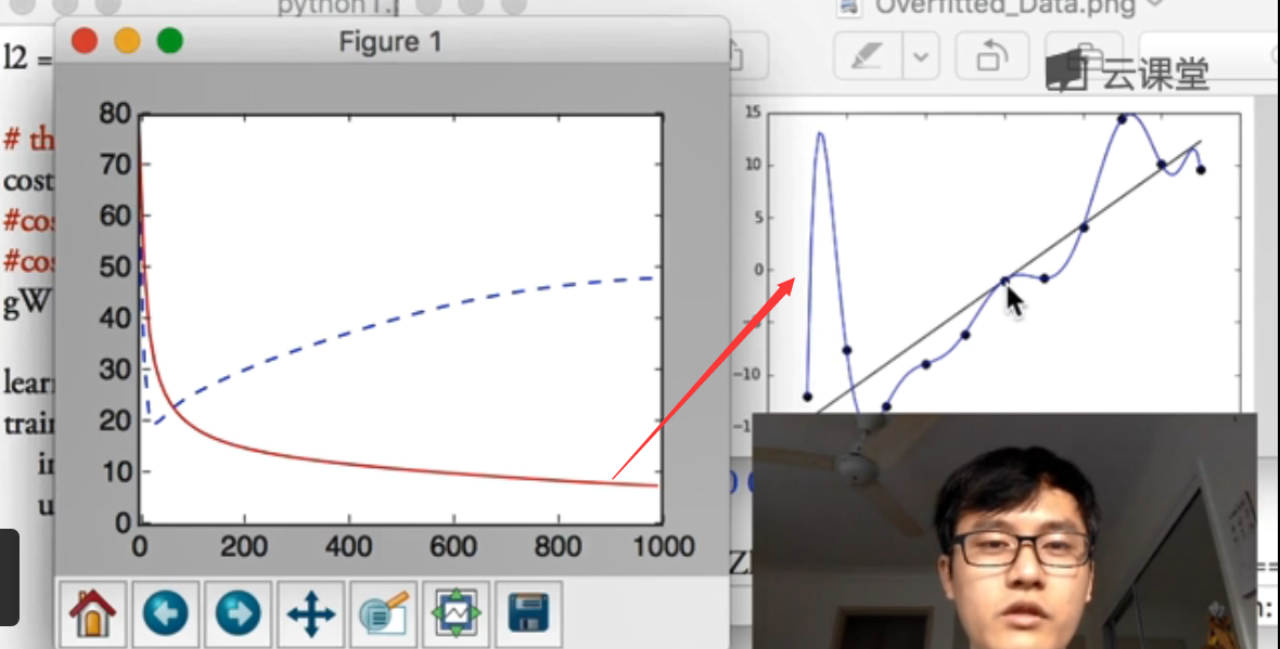
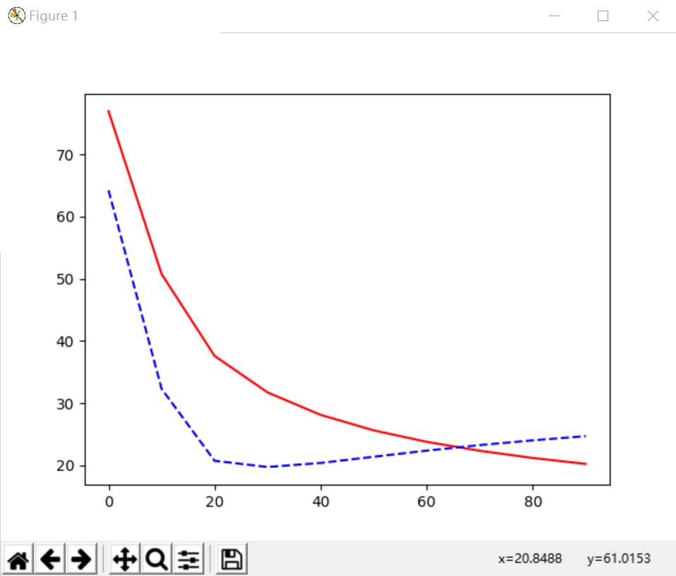
（1）Overfitting问题对应曲线，红色线为训练误差，蓝色虚线为测试结果，会发现预测的误差在不断变大。
    cost = T.mean(T.square(L2.outputs-y))

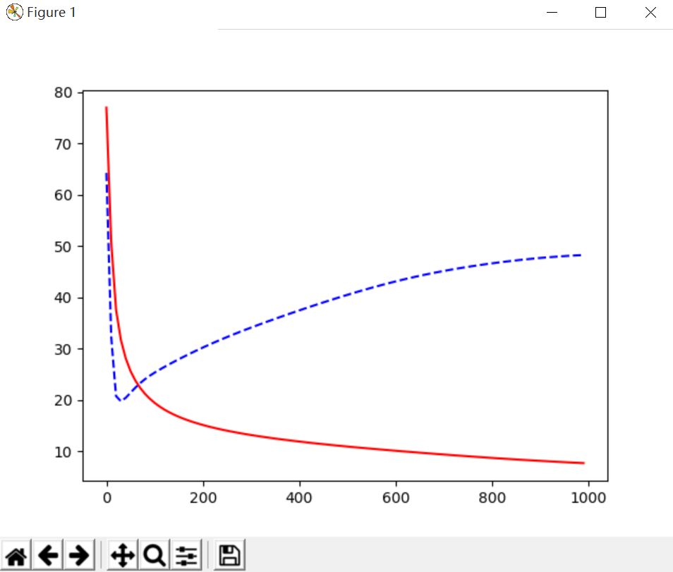
参考莫烦大神视频原图，对应的蓝色曲线就没有黑色直线预测效果好，也看看大神风貌吧，也推荐大家去学习，哈哈！

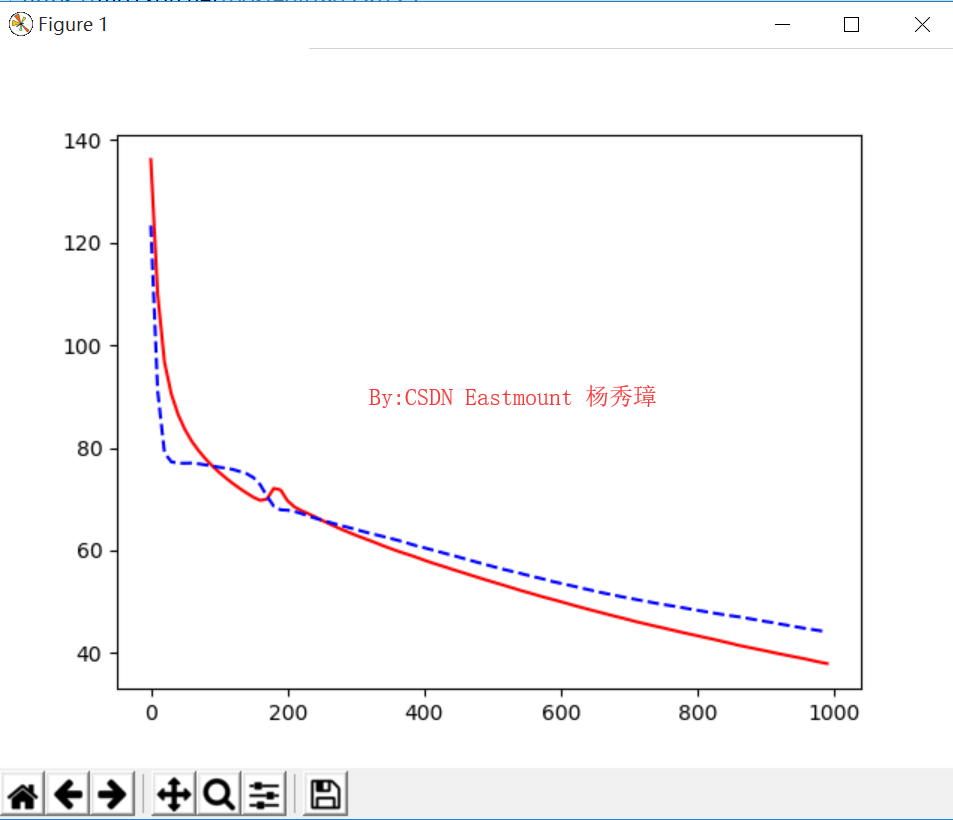
（2）L2 Regularization，通过正规化处理后的结果，发现预测结果和训练结果的误差变化基本一致，其效果更好。
    cost = T.mean(T.square(L2.outputs-y)) + 0.1*((L1.W**2).sum() + (L2.W**2).sum())

这里输出了1000个，而输出100个值如下所示：

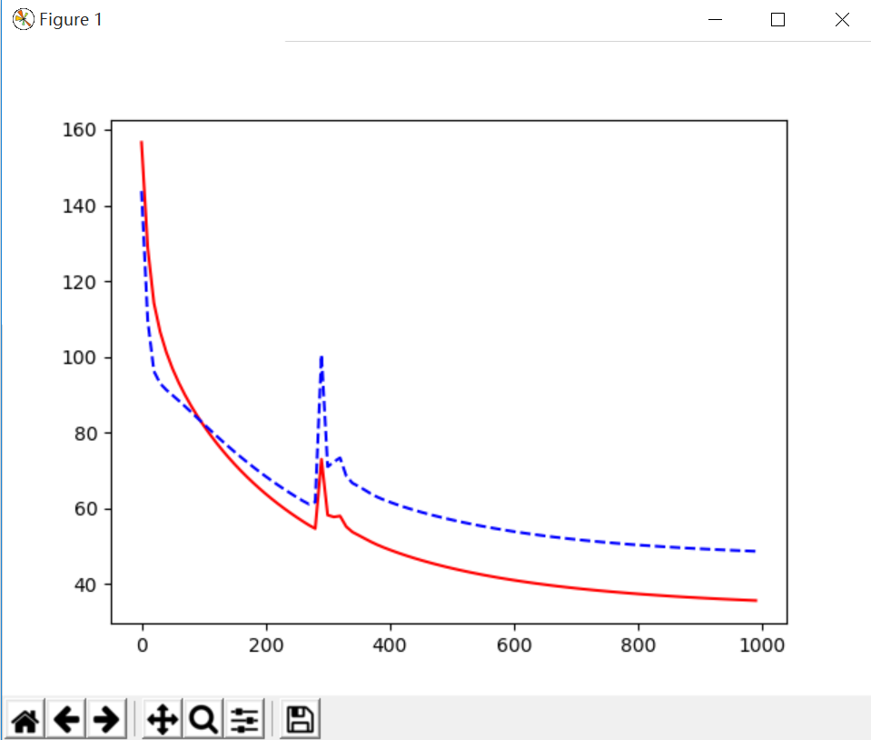
（3）L1 regularization输出结果如下图所示：
    cost = T.mean(T.square(L2.outputs-y)) + 0.1*(abs(L1.W).sum() + abs(L2.W).sum())

一个人如果总是自己说自己厉害，那么他就已经再走下坡路了，最近很浮躁，少发点朋友圈和说说吧，更需要不忘初心，砥砺前行。珍惜每一段学习时光，也享受公交车的视频学习之路，加油，最近兴起的傲娇和看重基金之心快离去吧，平常心才是更美，当然娜最美，早安。
原文出处