#矩阵操作与线性方程组 from numpy.linalg import * print (np.eye(3)) #他是一个3行3列的单位矩阵 list = np.array(([1, 2], [3, 4])) print (inv(list)) #逆矩阵 print (list.transpose()) # 转置矩阵 print (det(list)) #求行列式（算的是行列式的值） print (eig(list)) #特征值和特征向量 y = np.array(([5.], [7.])) {x+2y=5 3x+4y=7} print (solve(list, y)) #求list与y组成的二元一次方程组的解

**2. 优化（scipy.optimize）**

scipy.optimize模块提供了函数最值、曲线拟合和求根的算法。

该模块包括：

——多元标量函数的无约束和约束极小化(minimize)。使用多种算法(例如BFGS、Nder-Mead单纯形、Newton共轭梯度、COBYLA或SLSQP)

——全局(蛮力)优化例程。basinhopping, differential_evolution)

——最小二乘极小化(least_squares)和曲线拟合(curve_fit)算法

——标量单变量函数极小化(minimize_scalar)和根查找器(root_scalar)

——多元方程组求解器(root)使用多种算法(例如，混合鲍威尔、Levenberg-MarQuardt或大规模方法，如Newton-Krylov)

**无约束函数最值(以最小值为例)：**

导入模块：

```

from scipy.optimize import minimize

import numpy as np

```

在数学最优化中，Rosenbrock函数是一个用来测试最优化算法性能的非凸函数，由Howard Harry Rosenbrock在1960年提出。也称为Rosenbrock山谷或Rosenbrock香蕉函数，也简称为香蕉函数。

函数表达式（N是x的维数）：


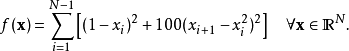
定义一个目标函数（Rosenbrock函数——香蕉函数）：

```

def rosen(x):

    """The Rosenbrock function"""

    return sum(100.0*(x[1:]-x[:-1]**2.0)**2.0+(1-x[:-1])**2.0)

x0 = np.array([1.3, 0.7, 0.8, 1.9, 1.2])

```

求解：

```

res = minimize(rosen, x0, method='nelder-mead', options={'xtol': 1e-8, 'disp': True})

 print（res.x）     #res.x是优化结果，返回一个ndarry

```

minimize(fun, x0[, args, method, jac, hess, …])   

fun——一个或多个变量的标量函数的最小化

x0——初始猜测值，相当于指定了N

method就是优化算法

Xtol是精度

disp指是否显示过程（True则显示）

过程与结果：

```

Optimization terminated successfully.

         Current function value: 0.000000

         Iterations: 339

         Function evaluations: 571

[1. 1. 1. 1. 1.]

```

**有约束函数最值（最小值为例）：**

导入模块：

```

from scipy.optimize import minimize

import numpy as np

```

定义函数：

f(x) = 2xy+2x-x^2^-2y^2^ 

偏导数：

2y+2-2x

2x-4y

```

def fun(x):

    return (2*x[0]*x[1]+2*x[0]-x[0]**2-2*x[1]**2)

def func_deriv(x):

    dfdx0 = (-2*x[0]+2*x[1]+2)

    dfdx1 = (2*x[0]-4*x[1])

    return np.ndarry([dfdx0,dfdx1])

```

约束条件(等于转化为=0和不等于转化为>=0):

3x^2^-y = 0

y-1>=0

```

cons = ({"type":"eq","fun":lambda x;np.ndarray([x[0]**3-x[1]]),"jac":lamda x;np.ndarray([3*(x[0]**2),-1])}

         ,{"type":"ineq","fun":lambda x;np.ndarray([x[1]-1]),"jac":lamda x;np.ndarray(0,1])})         

```

雅可比矩阵是函数的一阶偏导数以一定方式排列成的矩阵，其行列式称为雅可比行列式。

求解：

```

x0 = np.array([-1.0, 1.0])

>>> res = minimize(func, x0, method='SLSQP', jac=func_deriv,constraints=cons, options={'disp': True})       #顺序最小二乘规划(SLSQP)算法(method='SLSQP')

print(res.x)

```

结果：

```

x：array([1.0000009,1])

```

**优化器求根：**

导入模块：

```

from scipy.optimize import root

import numpy as np

```

定义函数：

x+2cos（x） = 0

```

def func(x):

    return x + 2 * np.cos(x)

```

求解和结果：

```

sol = root(func, 0.1)   #root（fun,x0)，fun为函数，x0是Initial guess.（初始猜测值）

print（sol.x） #优化（根）结果

>>array([-1.02986653])

print（sol.fun）     #目标函数的值

>>array([ -6.66133815e-16])

```

python之数据分析概述：

python数据分析大家族：

① numpy：数据结构基础

② scipy：强大的科学计算方法（矩阵分析、信号分析、数理分析....）

③ matplotlib：丰富的可视化套件（三维图、饼图、可视图等）

④ pandas：基础数据分析套件（表）

⑤ scikit-learn：强大的数据分析建模库（回归分析 、聚类分析）

⑥ keras：人工神经网络 

np.array 用来创建一个numpy数组。 np.shape 显示np数组属性 np.ndim 表示数组维度 np.dtype表示数组元素类型（如：int8，in16,float64等） np.itemsize表示数组元素所占字节大小，如float64占字节8位 np.size表示数组元素个数

#常用array操作 list = (np.arange(1, 11)) #产生一个1-11（不含11）的等差数列 list = (np.arange(1, 11)).reshape([2, 5]) # 变成两行五列数组 print (np.exp(list)) # list 的自然指数 print (np.exp2(list)) # list 的自然指数的平方 print (np.sqrt(list)) # list 的开方 print (np.square(list)) # list 的平方 print (np.sin(list)) # list 的正弦值 print (np.log(list)) # list 的对数值 print (np.vstack((list1,list2))) #将两个数组分成两行组成一个数组也就是以行连接，注意传的是个tuple print (np.hstack((list1,list2))) #将两个数组相连组成一个一维数组，传的是tup print (np.split(list1,n)) #将数组 list1 切分成n个子数组 print (np.copy(list1)) #对数组进行拷贝

print (np.zeros([2, 4]))#输出元素都为0的2行4列数组 print (np.ones([3, 5]))#输出元素都为1 的2行4列数组 print ("Rand:") print (np.random.rand(2, 4))#输出2行4列的随机数组 print (np.random.rand())#生成一个随机数 print (np.random.randint(1, 14, 5))#在1到14之间生成5个随机数 print (np.random.randn(2, 4))#输出2行4列标准正态分布随机数 print np.random.choice([10.20, 41])#在列表中的数随机选取一个 print (np.random.beta(1,10, 100))#生成一个1-10共100个beta数组

List每次处理对象会判断数据类型，可存放多种类数据，但维护成本较高

shape表示几行几列 ndim表示维数 dtype表示元素的数据类型 itemsize表示元素的大小，比如float就是8个字节 size表示元素组合总的个数

# 4. liner
from numpy.linalg import *
print np.eye(3) # 单位矩阵
lst = np.array([[1, 2],
                [3, 4]])
print "Inv:"
print inv(lst) # 矩阵的逆
print "T"
print lst.transpose() # 转置矩阵
print "Det:"
print det(lst) # 行列式
print eig(lst) # 特征值和特征向量，一个元组，两个array
y = np.array([[5], [7]])
print "Solve"
print solve(lst, y) # 解方程组 x+2y=5; 3x+4y=7

# 3. Some Array Opers
lst = np.arange(1, 11).reshape([2, 5]) # 5可以缺省为-1， 产生一个1-11（不含11）的等差数列
print lst
print "Exp"
print np.exp(lst)
print "Exp2"
print np.exp2(lst)
print "Sqrt"
print np.sqrt(lst)
print "sin"
print np.sin(lst)
print "log"
print np.log(lst)

lst = np.arange(1,25).reshape([3, 2, 4]) # 等差数列
# 即如下数组
lst = np.array([[[1, 2, 3, 4],
                 [5, 6, 7, 8]],
                [[9, 10, 11, 12],
                 [13, 14, 15, 16]],
                [[17, 18, 19, 20],
                 [21, 22, 23, 24]]])
print lst
print lst.sum()
# x为维度，x越大，深入程度越大。0：最外层，1：再往里深入一层，对各个元素操作
print lst.sum(axis=0) # 最外层共3个元素，第一个元素：[[1, 2, 3, 4], [5, 6, 7, 8]]
print lst.sum(axis=1) # 再深入一层，第一个元素：[1, 2, 3, 4]，第二个：[5, 6, 7, 8]
print lst.sum(axis=2) # 再深入一层，遍历[1, 2, 3, 4]求和得第一个元素。
print lst.max(), lst.min()
print lst.max(axis=2)
print lst.max(axis=1)
print lst.max(axis=0)

# 对两个数组操作
lst1 = np.array([10, 20, 30, 40])
lst2 = np.array([4, 3, 2, 1])
print "Add"
print lst1+lst2
print "Sub"
print lst1-lst2
print "Mul"
print lst1*lst2
print "Div"
print lst1/lst2
print "Square"
print lst1**2
print "Dot" # 点乘
print np.dot(lst1.reshape([2, 2]), lst2.reshape([2, 2]))

# numpy 中 array 追加 Concatenate
print "Concatenate"
print np.concatenate((lst1, lst2), axis=0) # 追加，更简单的追加如下
print np.vstack((lst1, lst2)) # 上下接起来，2行，垂直接起来
print np.hstack((lst1, lst2)) # 水平接起来
print np.split(lst1, 2) # 分割为两个数组
print np.copy(lst1) # 拷贝

fig = plt.figure()
ax = fig.add_subplot(3, 3, 1)
n = 128
X = np.random.normal(0, 1, n)
Y = np.random.normal(0, 1, n)
T = np.arctan2(Y, X)
# plt.axes([0.025, 0.025, 0.95, 0.95])
ax.scatter(X, Y, s=75, c=T, alpha=.5)
plt.xlim(-1.5, 1.5), plt.xticks([])
plt.ylim(-1.5, 1.5), plt.yticks([])
plt.axis()
plt.title("scatter")
plt.xlabel("x")
plt.ylabel("y")
# bar
fig.add_subplot(332)
n = 10
X = np.arange(n)
Y1 = (1 - X / float(n) * np.random.uniform(0.5, 1.0, n))
Y2 = (1 - X / float(n) * np.random.uniform(0.5, 1.0, n))

plt.bar(X, +Y1, facecolor="#9999ff", edgecolor="white")
plt.bar(X, -Y2, facecolor="#ff9999", edgecolor="white")
for x, y in zip(X, Y1):
    plt.text(x + 0.4, y + 0.05, '%.2f' % y, ha='center', va='bottom')
for x, y in zip(X, Y2):
    plt.text(x + 0.4, -y - 0.05, '%.2f' % y, ha='center', va='top')

# Pie
fig.add_subplot(333)
n = 20
Z = np.ones(n)
Z[- 1] *= 2
plt.pie(Z, explode=Z * .05, colors=['%f' % (i / float(n)) for i in range(n)],
        labels=['%.2f' % (i / float(n)) for i in range(n)])
plt.gca().set_aspect('equal')
plt.xticks(), plt.yticks([])

# polar
fig.add_subplot(334, polar=True)
n = 20
theta = np.arange(0.0, 2 * np.pi, 2 * np.pi / n)
radii = 10 * np.random.rand(n)
# plt.plot(theta,radii)
plt.polar(theta, radii)

# heatmap
fig.add_subplot(335)
from matplotlib import cm
data = np.random.rand(3, 3)
cmap = cm.Blues
map = plt.imshow(data, interpolation='nearest', cmap=cmap,
                 aspect='auto', vmin=0, vmax=1)
# 3D
from mpl_toolkits.mplot3d import Axes3D
ax = fig.add_subplot(336, projection="3d")
ax.scatter(1, 1, 3, s=100)

# hot map
fig.add_subplot(313)

def f(x, y):
    return (1 - x / 2 + x ** 5 + y ** 3) * np.exp(-x ** 2 - y ** 2)

n = 256
x = np.linspace(-3, 3, n)
y = np.linspace(-3, 3, n)
X, Y = np.meshgrid(x, y)
plt.contourf(X, Y, f(X, Y), 8, alpha=.75, cmap=plt.cm.hot)
plt.savefig("./fig.png")
plt.show()

1分58秒操作的这个后台怎么打开的

应该是对于二维矩阵而言, sum函数里面的axis是指定行或者列. axis=0的话是按列求和, axis=1是按行求和 如果没有axis参数的话就是全部元素求和 更高维度的矩阵的话axis可以看成指定的是维度 #常用array操作 list = (np.arange(1, 11)) #产生一个1-11（不含11）的等差数列 list = (np.arange(1, 11)).reshape([2, 5]) # 变成两行五列数组 print (np.exp(list)) # list 的自然指数 print (np.exp2(list)) # list 的自然指数的平方 print (np.sqrt(list)) # list 的开方 print (np.square(list)) # list 的平方 print (np.sin(list)) # list 的正弦值 print (np.log(list)) # list 的对数值 print (np.vstack((list1,list2))) #将两个数组分成两行组成一个数组也就是以行连接，注意传的是个tuple print (np.hstack((list1,list2))) #将两个数组相连组成一个一维数组，传的是tup print (np.split(list1,n)) #将数组 list1 切分成n个子数组 print (np.copy(list1)) #对数组进行拷贝

#numpy的其他操作 print("FFT:") print (np.fft.fft(np.array([1,1,1,1,1,1,1,]))) print (np.corrcoef([1, 0, 1],[0, 2, 1])) # 皮尔逊相关系数计算 print (np.poly1d([3,1,3])) # 生成一元多次函数

numpy (Numerical Python):数据结构基础

scipy:强大的科学计算方法（矩阵分析、信号分析、数理分析。。）

matplotlib：丰富的可视化套件

pandas：基础数据分析套件

scikit-learn：强大的数据分析建模库

keras：人工神经网络

def main():
    # Data Structure
    s=pd.Series([i*2 for i in range(1,11)])
    print(type(s))
    dates=pd.date_range("20170301",periods=8)
    df=pd.DataFrame(np.random.rand(8,5),index=dates,columns=list("ABCDE"))
    print(df)
    df = pd.DataFrame({"A": 1, "B": pd.Timestamp("20170301"), "C": pd.Series(1, index=list(range(4)), dtype="float32"),
                       "D": np.array([3]*4, dtype="float32"), "E": pd.Categorical(["police", "student", "teacher", "doctor"])})
    print(df)